Centauri Dreams
Imagining and Planning Interstellar Exploration
JWST Catch: Directly Imaged Planet Candidate
We have so few exoplanets that can actually be seen rather than inferred through other data that the recent news concerning the star TWA 7 resonates. The James Webb Space Telescope provided the data on a gap in one of the rings found around this star, with the debris disk itself imaged by the European Southern Observatory’s Very Large Telescope as per the image below. The putative planet is the size of Saturn, but that would make it the planet with the smallest mass ever observed through direct imaging.
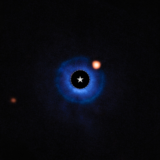
Image: Astronomers using the NASA/ESA/CSA James Webb Space Telescope have captured compelling evidence of a planet with a mass similar to Saturn orbiting the young nearby star TWA 7. If confirmed, this would represent Webb’s first direct image discovery of a planet, and the lightest planet ever seen with this technique. Credit: © JWST/ESO/Lagrange.
Adding further interest to this system is that TWA 7 is an M-dwarf, one whose pole-on dust ring was discovered in 2016, so we may have an example of a gas giant in formation around such a star, a rarity indeed. The star is a member of the TW Hydrae Association, a grouping of young, low-mass stars sharing a common motion and, at about a billion years old, a common age. As is common with young M-dwarfs, TWA 7 is known to produce strong X-ray flares.
We have the French-built coronagraph installed on JWST’s MIRI instrument to thank for this catch. Developed through the Centre national de la recherche scientifique (CNRS), the coronagraph masks starlight that would otherwise obscure the still unconfirmed planet. It is located within a disk of debris and dust that is observed ‘pole on,’ meaning the view as if looking at the disk from above. Young planets forming in such a disk are hotter and brighter than in developed systems, much easier to detect in the mid-infrared range.
In the case of TWA 7, the ring-like structure was obvious. In fact, there are three rings here, the narrowest of which is surrounded by areas with little matter. It took observations to narrow down the planet candidate, but also simulations that produced the same result, a thin ring with a gap in the position where the presumed planet is found. Which is to say that the planet solution makes sense, but we can’t yet call this a confirmed exoplanet.
The paper in Nature runs through other explanations for this object, including a distant dwarf planet in our own Solar System or a background galaxy. The problem with the first is that no proper motion is observed here, as would be the case even with a very remote object like Eris or Sedna, both of which showed discernible proper motion at the time of their discovery. As to background galaxies, there is nothing reported at optical or near-infrared wavelengths, but the authors cannot rule out “an intermediate-redshift star-forming [galaxy],” although they calculate that probability at about 0.34%.
The planet option seems overwhelmingly likely, as the paper notes:
The low likelihood of a background galaxy, the successful fit of the MIRI flux and SPHERE upper limits by a 0.3-MJ planet spectrum and the fact that an approximately 0.3-MJ planet at the observed position would naturally explain the structure of the R2 ring, its underdensity at the planet’s position and the gaps provide compelling evidence supporting a planetary origin for the observed source. Like the planet β Pictoris b, which is responsible for an inner warp in a well-resolved—from optical to millimetre wavelengths—debris disk, TWA 7b is very well suited for further detailed dynamical modelling of disk–planet interactions. To do so, deep disk images at short and millimetre wavelengths are needed to constrain the disk properties (grain sizes and so on).
So we have a probable planet in formation here, a hot, bright object that is at least 10 times lighter than any exoplanet that has ever been directly imaged. Indeed, the authors point out something exciting about JWST’s capabilities. They argue that planets as light as 25 to 30 Earth masses could have been detected around this star. That’s a hopeful note as we move the ball forward on detecting smaller exoplanets down to Earth-class with future instruments.
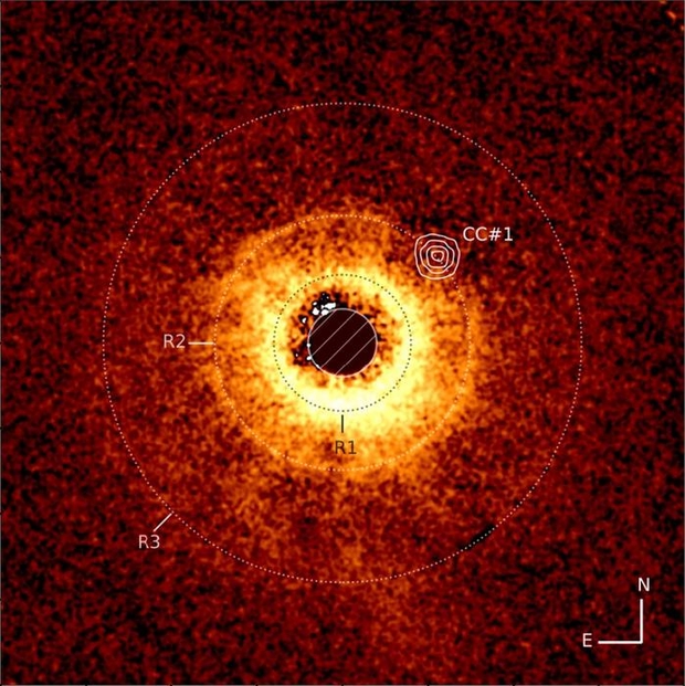
Image: The disk around the star TWA 7 recorded using ESO’s Very Large Telescope’s SPHERE instrument. The image captured with JWST’s MIRI instrument is overlaid. The empty area around TWA 7 B is in the R2 ring (CC #1). Credit: © JWST/ESO/Lagrange.
The paper is Lagrange et al., “Evidence for a sub-Jovian planet in the young TWA 7 disk,” Nature 25 June 2025 (full text).
Addendum: I’ve just become aware of Crotts et al., “Follow-Up Exploration of the TWA 7 Planet-Disk System with JWST NIRCam,” accepted for publication at Astrophysical Journal Letters (preprint). From which this:
…we present new observations of the TWA 7 system with JWST/NIRCam in the F200W and F444W filters. The disk is detected at both wavelengths and presents many of the same substructures as previously imaged, although we do not robustly detect the southern spiral arm. Furthermore, we detect two faint potential companions in the F444W filter at the 2-3σ level. While one of these companions needs further followup to determine its nature, the other one coincides with the location of the planet candidate imaged with MIRI, providing further evidence that this source is a sub-Jupiter mass planet companion rather than a background galaxy. Such discoveries make TWA 7 only the second system, after β Pictoris, in which a planet predicted by the debris disk morphology has been detected.

Interstellar Flight: Perspectives and Patience
This morning’s post grows out of listening to John Coltrane’s album Sun Ship earlier in the week. If you’re new to jazz, Sun Ship is not where you want to begin, as Coltrane was already veering in a deeply avant garde direction when he recorded it in 1965. But over the years it has held a fascination for me. Critic Edward Mendelowitz called it “a riveting glimpse of a band traveling at warp speed, alternating shards of chaos and beauty, the white heat of virtuoso musicians in the final moments of an almost preternatural communion…” McCoy Tyner’s piano is reason enough to listen.

As music often does for me, Sun Ship inspired a dream that mixed the music of the Coltrane classic quartet (Tyner, Jimmy Garrison and Elvin Jones) with an ongoing story. The Parker Solar Probe is, after all, a real ‘sun ship,’ one that on December 24 of last year made its closest approach to the Sun. Moving inside our star’s corona is a first – the craft closed to within 6.1 million kilometers of the solar surface.
When we think of human technology in these hellish conditions, those of us with an interstellar bent naturally start musing about ‘sundiver’ trajectories, using a solar slingshot to accelerate an outbound spacecraft, perhaps with a propulsive burn at perihelion. The latter option makes this an ‘Oberth maneuver’ and gives you a maximum outbound kick. Coltrane might have found that intriguing – one of his later albums was, after all, titled Interstellar Space.
I find myself musing on speed. The fastest humans have ever moved is the 39,897 kilometers per hour that the trio of Apollo 10 astronauts – Tom Stafford, John Young and Eugene Cernan – experienced on their return to Earth in 1969. The figure translates into just over 11 kilometers per second, which isn’t half bad. Consider that Voyager 1 moves at 17.1 km/sec, and it’s the fastest object we’ve yet been able to send into deep space.
True, New Horizons has the honor of being the fastest craft immediately after launch, moving at over 16 km/sec and thus eclipsing Voyager 1’s speed before the latter’s gravity assists. But New Horizons has since slowed as it climbs out of the Sun’s gravitational well, now making on the order of 14.1 km/sec, with no gravity assists ahead. Wonderfully, operations continue deep in the Kuiper Belt.
It’s worth remembering that at the beginning of the 20th Century, a man named Fred Mariott became the fastest man alive when he managed 200 kilometers per hour in a steam-powered car (and somehow survived). Until we launched the Parker Solar Probe, the two Helios missions counted as the fastest man-made objects, moving in elliptical orbits around the Sun that reached 70 kilometers per second. Parker outdoes this: At perihelion in late 2024, it managed 191.2 km/sec, so it now holds velocity as well as proximity records.
191.2 kilometers per second gets you to Proxima Centauri in something like 6,600 years. A bit long even for the best equipped generation ship, I think you’ll agree. Surely Heinlein’s ‘Vanguard,’ the starship in Orphans of the Sky was moving at a much faster clip even if its journey took many centuries to reach the same star. I don’t think Heinlein ever let us know just how many. Of course, we can’t translate the Parker spacecraft’s infalling velocity into comparable numbers on an outbound journey, but it’s fun to speculate on what these numbers imply.
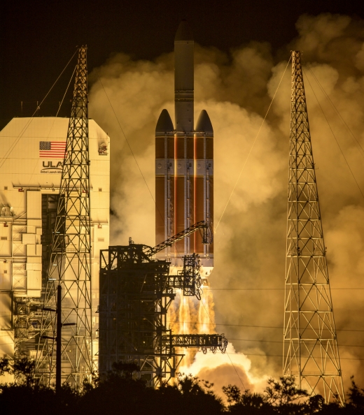
Image: The United Launch Alliance Delta IV Heavy rocket launches NASA’s Parker Solar Probe to touch the Sun, Sunday, Aug. 12, 2018, from Launch Complex 37 at Cape Canaveral Air Force Station, Florida. Parker Solar Probe is humanity’s first-ever mission into a part of the Sun’s atmosphere called the corona. The mission continues to explore solar processes that are key to understanding and forecasting space weather events that can impact life on Earth. It also gives a nudge to interstellar dreamers. Credit: NASA/Bill Ingalls.
Speaking of Voyager 1, another interesting tidbit relates to distance: In 2027, the perhaps still functioning spacecraft will become the first human object to reach one light-day from the Sun. That’s just a few steps in terms of an interstellar journey, but nonetheless meaningful. Currently radio signals take over 23 hours to reach the craft, with another 23 required for a response to be recorded on Earth. Notice that 2027 will also mark the 50th year since the two Voyagers were launched. January 28, 2027 is a day to mark in your calendar.
Since we’re still talking about speeds that result in interstellar journeys in the thousands of years, it’s also worth pointing out that 11,000 work-years were devoted to the Voyager project through the Neptune encounter in 1989, according to NASA. That is roughly the equivalent of a third of the effort estimated to complete the Great Pyramid at Giza during the reign of Khufu, (~2580–2560 BCE) in the fourth dynasty of the Old Kingdom. That’s also a tidbit from NASA, telling me that someone there is taking a long term perspective.
Coltrane’s Sun Ship has also led me to the ‘solar boat’ associated with Khufu. The vessel was found sealed in a space near the Great Pyramid and is the world’s oldest intact ship, buried around 2500 BCE. It’s a ritual vessel that, according to archaeologists, was intended to carry the resurrected Khufu across the sky to reach the Sun god the Egyptians called Ra.
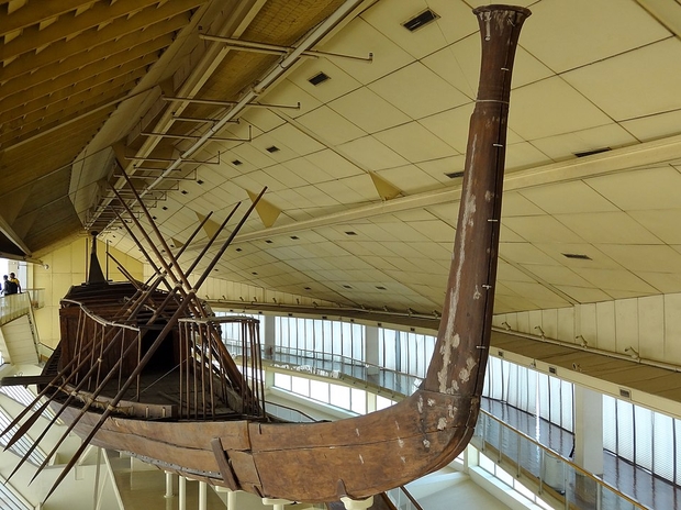
Image: The ‘sun ship’ associated with the Egyptian king Khufu, in the pre-Pharaonic era of ancient Egypt. Credit: Olaf Tausch, CC BY 3.0. Wikimedia Commons.
My solar dream reminds me that interstellar travel demands reconfiguring our normal distance and time scales as we comprehend the magnitude of the problem. While Voyager 1 will soon reach a distance of 1 light day, it takes light 4.2 years to reach Proxima Centauri. To get around thousand-year generation ships, we are examining some beamed energy solutions that could drive a small sail to Proxima in 20 years. We’re a long way from making that happen, and certainly nowhere near human crew capabilities for interstellar journeys.
But breakthroughs have to be imagined before they can be designed. Our hopes for interstellar flight exercise the mind, forcing the long view forward and back. Out of such perspectives dreams come, and one day, perhaps, engineering.
TFINER: Ramping Up Propulsion via Nuclear Decay
Sometimes all it takes to spawn a new idea is a tiny smudge in a telescopic image. What counts, of course, is just what that smudge implies. In the case of the object called ‘Oumuamua, the implication was interstellar, for whatever it was, this smudge was clearly on a hyperbolic orbit, meaning it was just passing through our Solar System. Jim Bickford wanted to see the departing visitor up close, and that was part of the inspiration for a novel propulsion concept.

Now moving into a Phase II study funded by NASA’s Innovative Advanced Concepts office (NIAC), the idea is dubbed Thin-Film Nuclear Engine Rocket (TFINER). Not the world’s most pronounceable acronym, but if the idea works out, that will hardly matter. Working at the Charles Stark Draper Laboratory, a non-profit research and development company in Cambridge MA, Bickford is known to long-time Centauri Dreams readers for his work on naturally occurring antimatter capture in planetary magnetic fields. See Antimatter Acquisition: Harvesting in Space for more on this.
Image: Draper Laboratory’s Jim Bickford, taking a deep space propulsion concept to the next level. Credit: Charles Stark Draper Laboratory.
Harvesting naturally occurring antimatter in space offers some hope of easing one of the biggest problems of such propulsion strategies, namely the difficulty in producing enough antimatter to fuel an engine. With the Thin Film Nuclear Engine Rocket, Bickford again tries to change the game. The notion is to use energetic radioisotopes in thin layers, allowing their natural decay products to propel a spacecraft. The proper substrate, Bickford believes, can control the emission direction, and the sail-like system packs a punch: Velocity changes on the order of 100 kilometers per second using mere kilograms of fuel.
I began this piece talking about ‘Oumuamua, but that’s just for starters. Because if we can create a reliable propulsion system capable of such tantalizing speed. we can start thinking about mission targets as distant as the solar gravitational focus, where extreme magnifications become possible. Because the lensing effect for practical purposes begins at 550 AU and continues with a focal line to infinity, we are looking at a long journey. Bear in mind that Voyager 1, our most distant working spacecraft, has taken almost half a century to reach, as of now, 167 AU. To image more than one planet at the solar lens, we’ll also need a high degree of maneuverability to shift to multiple exoplanetary systems.
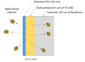
Image: This is Figure 3-1 from the Phase 1 report. Caption: Concept for the thin film thrust sheet engine. Alpha particles are selectively emitted in one direction at approximately 5% of the speed of light. Credit: NASA/James Bickford.
So we’re looking at a highly desirable technology if TFINER can be made to work, one that could offer imaging of exoplanets, outer planet probes, and encounters with future interstellar interlopers. Bickford’s Phase 1 work will be extended in the new study to refine the mission design, which will include thruster experiments as well as what the Phase II summary refers to as ‘isotope production paths’ while also considering opportunities for hybrid missions that could include the Oberth ‘solar dive’ maneuver. More on that last item soon, because Bickford will be presenting a paper on the prospect this summer.
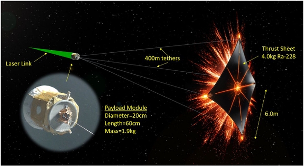
Image: Artist concept highlighting the novel approach proposed by the 2025 NIAC awarded selection of the TFINER concept. This is the baseline TFINER configuration used in the system analysis. Credit: NASA/James Bickford.
But let’s drop back to the Phase I study. I’ve been perusing Bickford’s final report. Developing out of Wolfgang Moeckel’s work at NASA Lewis in the 1970s, the TFINER design uses thin sheets of radioactive elements. The solution leverages exhaust velocities for alpha particle decays that can exceed 5 percent of the speed of light. You’ll recall my comment on space sails in the previous post, where we looked at the advantage of inflatable components to make sails more scalable. TFINER is more scalable still, with changes to the amount of fuel and sheet area being key variables.
Let’s begin with a ~10-micron thick Thorium-228 radioisotope film, with each sheet containing three layers, integrating the active radioisotope fuel layer in the middle. Let me quote from the Phase I report on this:
It must be relatively thin to avoid substantial energy losses as the alpha particles exit the sheet. A thin retention film is placed over this to ensure that the residual atoms do not boil off from the structure. Finally, a substrate is added to selectively absorb alpha emission in the forward direction. Since decay processes have no directionality, the substrate absorber produces the differential mass flow and resulting thrust by restricting alpha particle trajectories to one direction.
The TFINER baseline uses 400 meter tethers to connect the payload module. The sheet’s power comes from Thorium-228 decay (alpha decay) — the half-life is 1.9 years. We get a ‘decay cascade chain’ that produces daughter products – four additional alpha emissions result with half-lives ranging from 300 ns to 3 days. The uni-directional thrust is produced thanks to the beryllium absorber (~35-microns thick) that coats one side of the thin film to capture emissions moving forward. Effective thrust is thus channeled out the back.
Note as well the tethers in the illustration, necessary to protect the sensor array and communications component to minimize the radiation dose. Manipulation of the tethers can control trajectory on single-stage missions to deep space targets. Reconfiguring the thrust sheet is what makes the design maneuverable, allowing thrust vectoring, even as longer half-life isotopes can be deployed in the ‘staged’ concept to achieve maximum velocities for extended missions.
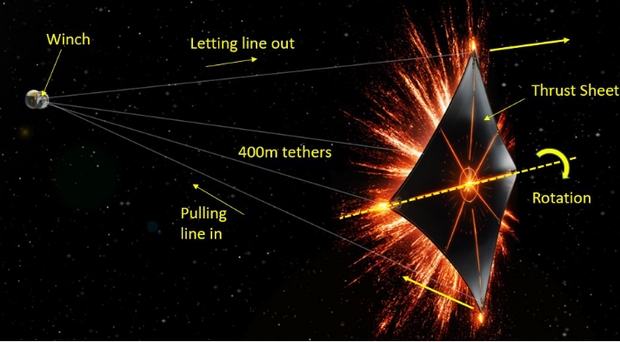
Image: This is Figure 7-8 from the report. Caption: Example thrust sheet rotation using tether control. Credit: NASA/James Bickford.
From the Phase I report:
The payload module is connected to the thrust sheet by long tethers. A winch on the payload module can individually pull-in or let-out line to manipulate the sail angle relative to the payload. The thrust sheet angle will rotate the mean thrust vector and operate much like trimming the sail of a boat. Of course, in this case, the sail (sheet) pressure comes from the nuclear exhaust rather than the wind
It’s hard to imagine the degree of maneuverability here being replicated in any existing propulsion strategy, a big payoff if we can learn how to control it:
This approach allows the thrust vector to be rotated relative to the center of mass and velocity vector to steer the spacecraft’s main propulsion system. However, this is likely to require very complex controls especially if the payload orientation also needs to be modified. The maneuvers would all be slow given the long lines lengths and separations involved.
Spacecraft pointing and control is an area as critical as the propulsion system. The Phase I report goes into the above options as well as thrust vectoring through sheets configured as panels that could be folded and adjusted. The report also notes that thermo-electrics within the substrate may be used to generate electrical power, although a radioisotope thermal generator integrated with the payload may prove a better solution. The report offers a good roadmap for the design refinement of TFINER coming in Phase II.
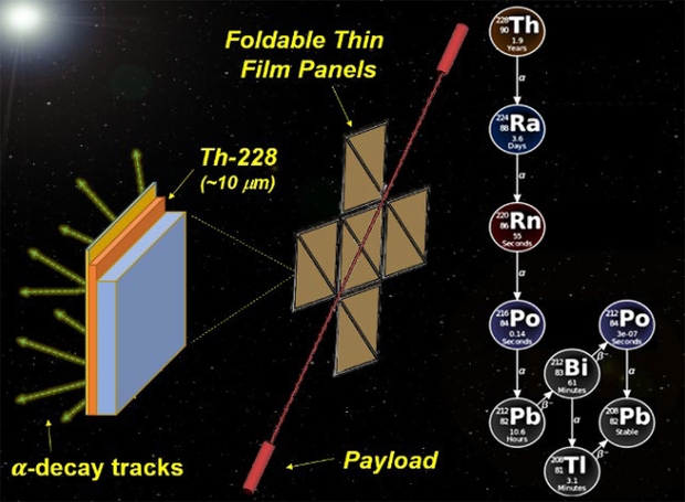
Image: TFINER imaged as in the Phase I study using a panel configuration. Credit: NASA/James Bickford.
The baseline TFINER concept considered in the report deploys 30 kg of Thorium-228 in a sheet area measuring over 250 square meters, a configuration capable of providing a delta-v of 150 km/s to a 30 kg payload. Bickford’s emphasis on maneuverability is well taken. A mission to the solar gravitational focus could take advantage of this capability by aligning with not just one but multiple targets through continuing propulsive maneuvers. Isotopes with a longer half-life (Bickford has studied Actinium-227, but other isotopes are possible) can provide for ‘staged’ combined architectures allowing still longer mission timeframes. A high-flux particle accelerator is assumed as the best production pathway to create the necessary isotopes.
Clearly we’re in the early stages of TFINER, but what an exciting concept. To return to ‘Oumuamua, the report notes that a mission to study it “…is not possible without the ability to slow down and perform a search along the trajectory since the uncertainty bubble in its trajectory is larger than the range of any sensors that would work during a flyby. The isotope fuel can be chosen to optimize for higher accelerations early in the mission or longer half-life options for extended missions.” As the Phase II report lays out the development path, questions of fuel production and substrate optimization will be fully explored.
I asked Dr. Bickford about how the Phase II study will proceed. In an email on Wednesday, he pointed to continuing analysis of the thrust sheet, fuel production and spacecraft design, which should involve potential mission architectures. But he passed along several other points of interest:
- Northwestern and Yale Universities have joined the team to operate a ~1 cm2 scale thruster demonstration to validate the force models and better understand the sheet’s electrical charging behavior.
- Draper Laboratory has expanded its work with Los Alamos National Laboratory to explore novel production approaches including new particle accelerators and fuel production architectures.
- ”We’ve added NASA MSFC as consultants to explore hybrid mission architectures which exploit solar pressure during the close solar flyby of an Oberth maneuver.”
Concepts like TFINER push the envelope in the kind of ways that pay off not only in a bank of new technical knowledge but novel technologies that will bear on how we explore the Solar System and eventually go beyond it. I’m reminded of Steve Howe and Gerald Jackson’s antimatter sail concept, which produces fission by allowing antimatter, stored probably as antihydrogen, to interact with a sheet of U-238 coated with carbon (see Antimatter and the Sail). TFINER uses no antimatter, but in both cases we have what looks like a sail surface being reinvented to offer missions that could put exotic targets within reach.
The other reason the antimatter sail comes to mind is that Jim Bickford is the man who reminded us how much naturally occurring antimatter may be available for harvest in the Solar System. The Howe/Jackson concept could work with milligrams of antimatter, which is conceivably available trapped in planetary magnetic fields, including that of Earth. In earlier work, Bickford has calculated that about a kilogram of antiprotons enter our Solar System every second, and any planet with a strong magnetic field is fair game for collection.
We hammer away at propulsion issues hoping for the breakthrough that will get us to the solar gravitational lens and the outer planets with much shorter mission timelines than available today. The thought of catching an interstellar interloper like ‘Oumuamua adds spice to the TFINER concept as the work continues. I look with great interest in the direction Bickford is taking with the Oberth maneuver, which we’ll be discussing further this summer.
Inflatable Technologies for Deep Space
One idea for deep space probes that resurfaces every few years is the inflatable sail. We’ve seen keen interest especially since Breakthrough Starshot’s emergence in 2016 in meter-class sails, perhaps as small as four meters to the side. But if we choose to work with larger designs, sails don’t scale well. Increase sail area and problems of mass arise thanks to the necessary cables between sail and payload. An inflatable beryllium sail filled with a low-pressure gas like hydrogen avoids this problem, with payload mounted on the space-facing surface. Such sails have already been analyzed in the literature (see below).
Roman Kezerashvili (City University of New York), in fact, recently analyzed an inflatable torus-shaped sail with a twist, one that uses compounds incorporated into the sail material itself as a ‘propulsive shell’ that can take advantage of desorption produced by a microwave beam or a close pass of the Sun. Laser beaming also produces this propulsive effect but microwaves are preferable because they do not damage the sail material. Kezerashvili has analyzed carbon in the sail lattice in solar flyby scenarios. The sail is conceived as “a thin reflective membrane attached to an inflatable torus-shaped rim.”
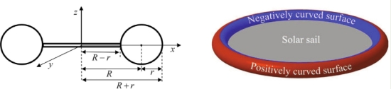
Image: This is Figure 1 from the paper. Credit: Kezerashvili et al.
Inflatable sails go back to the late 1980s. Joerg Strobl published a paper on the concept in the Journal of the British Interplanetary Society, and it received swift follow-up in a series of studies in the 1990s examining an inflatable radio telescope called Quasat. A series of meetings involving Alenia Spazio, an Italian aerospace company based in Turin, took the idea further. In 2018, Claudio Maccone, Greg Matloff, and NASA’s Les Johnson joined Kezerashvili in analyzing inflatable technologies for missions as challenging as a probe to the Oort Cloud.
Indeed, working with Joseph Meany in 2023, Matloff would also describe an inflatable sail using aerograpahite and graphene, enabling higher payload mass and envisioning a ‘sundiver’ trajectory to accelerate an Alpha Centauri mission. The conception here is for a true interstellar ark carrying a crew of several hundred, using a sail with radius of 764 kilometers on a 1300 year journey. So the examination of inflatable sails in varying materials is clearly not slowing down.
The Inflatable Starshade
But there are uses for inflatable space structures that go beyond outer system missions. I see that they are now the subject of a NIAC Phase I study by John Mather (NASA GSFC) that puts a new wrinkle into the concept. Mather’s interest is not propulsion but an inflatable starshade that, in various configurations, could work either with the planned Habitable Worlds Observatory or an Extremely Large Telescope like the 39 m diameter European Extremely Large Telescope now being built in Chile. Starshades are an alternative to coronagraph technologies that suppress light from a star to reveal its planetary companions.
Inflatables may well be candidates for any kind of large space structure. Current planning on the Habitable Worlds Observatory, scheduled for launch no earlier than the late 2030s, includes a coronagraph, but Mather thinks the two technologies offer useful synergies. Here’s a quote from the study summary:
A starshade mission could still become necessary if: A. The HWO and its coronagraph cannot be built and tested as required; B. The HWO must observe exoplanets at UV wavelengths, or a 6 m HWO is not large enough to observe the desired targets; C. HWO does not achieve adequate performance after launch, and planned servicing and instrument replacement cannot be implemented; D. HWO observations show us that interesting exoplanets are rare, distant, or are hidden by thick dust clouds around the host star, or cannot be fully characterized by an upgraded HWO; or E. HWO observations show that the next step requires UV data, or a much larger telescope, beyond the capability of conceivable HWO coronagraph upgrades.
So Mather’s idea is also meant to be a kind of insurance policy. It’s worth pointing out that coronagraphs are well studied and compact, while starshade technologies are theoretically sound but untested in space. But as the summary mentions, work at ultraviolet wavelengths is out of the coronagraph’s range. To get into that part of the spectrum, pairing Habitable Worlds Observatory with a 35-meter starshade seems the only option. This conceivably would allow a relaxation of some HWO optical specs, and thus lower the overall cost. The NIAC study will explore these options for a 35-meter as well as a 60-meter starshade.
I mentioned the possibility of combining a starshade with observations through an Extremely Large Telescope, an eye-widening notion that Mather proposed in a 2022 NIAC Phase I study. The idea here is to place the starshade in an orbit that would match position and velocity with the telescope, occulting the star to render the planets more visible. This would demand an active propulsion system to maintain alignment during the observation, while also making use of the adaptive optics already built into the telescope to suppress atmospheric distortion. The mission is called Hybrid Observatory for Earth-like Exoplanets.
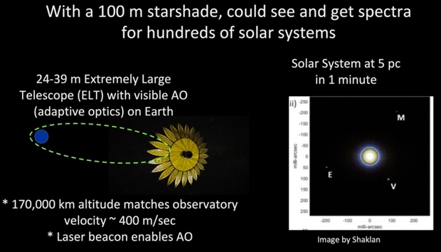
Image: Artist concept highlighting the novel approach proposed by the 2025 NIAC awarded selection of Inflatable Starshade for Earthlike Exoplanets concept. Credit: NASA/John Mather.
As discussed earlier, mass considerations play into inflatable designs. In the HOEE study, Mather referred to his plan “to cut the starshade mass by more than a factor of 10. There is no reason to require thousands of kg to support 400 kg of thin membranes.” His design goal is to create a starshade that can be assembled in space, thus avoiding launch and deployment issues. All this to create what he calls “the most powerful exoplanet observatory yet proposed.”
You can see how the inflatable starshade idea grows out of the hybrid observatory study. By experimenting with designs producing the needed strength, stiffness, stability and thermal requirements and the issues raised by bonding large sheets of materials of the requisite strength, the mass goals may be realized. So the inflatable sail option once again morphs into a related design, one optimized as an adjunct to an exoplanet observatory, provided this early work can lead to a solution that could benefit both astronomy and sails.
The paper on inflatable beryllium sails is Matloff, G. L., Kezerashvili, R. Ya., Maccone, C. and Johnson, L., “The Beryllium Hollow-Body Solar Sail: Exploration of the Sun’s Gravitational Focus and the Inner Oort Cloud”, arXiv:0809.3535v1 [physics.space-ph] 20 Sep 2008. The later Kezerashvili paper is Kezerashvili et al., “A torus-shaped solar sail accelerated via thermal desorption of coating,” Advances in Space Research Vol. 67, Issue 9 (2021), pp. 2577-2588 (abstract). The Matloff and Meany paper on an Alpha Centauri interstellar ark is ”Aerographite: A Candidate Material for Interstellar Photon Sailing,” JBIS Vol. 77 (2024) pp. 142-146. Abstract. Thanks to Thomas Mazanec and Antonio Tavani for the pointer to Mather’s most recent NIAC study.
Odd Couple: Gas Giants and Red Dwarfs
The assumption that gas giant planets are unlikely around red dwarf stars is reasonable enough. A star perhaps 20 percent the mass of the Sun should have a smaller protoplanetary disk, meaning sufficient gas and dust to build a Jupiter-class world are lacking. The core accretion model (a gradual accumulation of material from the disk) is severely challenged. Moreover, these small stars are active in their extended youth, sending out frequent flares and strong stellar winds that should dissipate such a disk quickly. Gravitational instabilities within the disk are one possible alternative.
Planet formation around such a star must be swift indeed, which accounts for estimates as low as 1 percent of such stars having a gas giant in the system. Exceptions like GJ 3512 b, discovered in 2019, do occur, and each is valuable. Here we have a giant planet, discovered through radial velocity methods, orbiting a star a scant 12 percent of the Sun’s mass. Or consider the star GJ 876, which has two gas giants, or the exoplanet TOI-5205 b, a transiting gas giant discovered in 2023. Such systems leave us hoping for more examples to begin to understand the planet forming process in such a difficult environment.
Let me drop back briefly to a provocative study from 2020 by way of putting all this in context before we look at another such system that has just been discovered. In this earlier work, the data were gathered at the Atacama Large Millimeter/submillimeter Array (ALMA), taken at a wavelength of 0.87 millimeters. The team led by Nicolas Kurtovic (Max Planck Institute for Astronomy, Heidelberg) found evidence of ring-like structures in protoplanetary disks that extend between 50 and 90 AU out.

Image: This is a portion of Figure 2 from the paper, which I’m including because I doubt most of us have seen images of a red dwarf planetary disk. Caption: Visibility modeling versus observations of our sample. From left to right: (1) Real part of the visibilities after centering and deprojecting the data versus the best fit model of the continuum data, (2) continuum emission of our sources where the scale bar represents a 10 au distance, (3) model image, (4) residual map (observations minus model), (5) and normalized, azimuthally averaged radial profile calculated from the beam convolved images in comparison with the model without convolution (purple solid line) and after convolution (red solid line). In the right most plots, the gray scale shows the beam major axis. Credit: Kurtovic et al.
Gaps in these rings, possibly caused by planetary embryos, would accommodate planets of the Saturn class, and the researchers find that gaps formed around three of the M-dwarfs in the study. The team suggests that ‘gas pressure bumps’ develop to slow the inward migration of the disk, allowing such giant worlds to coalesce. It’s an interesting possibility, but we’re still early in the process of untangling how this works. For more, see How Common Are Giant Planets around Red Dwarfs?, a 2021 entry in these pages.
Now we learn of TOI-6894 b, a transiting gas giant found as part of Edward Bryant’s search for such worlds at the University of Warwick and the University of Liège. An international team of astronomers confirmed the find using telescopes at the SPECULOOS and TRAPPIST projects. The work appears in Nature Astronomy (citation below). Here’s Bryant on the scope of the search for giant M-dwarf planets:
“I originally searched through TESS observations of more than 91,000 low-mass red-dwarf stars looking for giant planets. Then, using observations taken with one of the world’s largest telescopes, ESO’s VLT, I discovered TOI-6894 b, a giant planet transiting the lowest mass star known to date to host such a planet. We did not expect planets like TOI-6894b to be able to form around stars this low-mass. This discovery will be a cornerstone for understanding the extremes of giant planet formation.”
TOI-6894 b has a radius only a little larger than Saturn, although it has only about half of Saturn’s mass. What adds spice to this particular find is that the host star is the lowest mass star found to have a transiting giant planet. In fact, TOI-6894 is only 60 percent the size of the next smallest red dwarf with a transiting gas giant. Given that 80 percent of stars in the Milky Way are red dwarfs, determining an accurate percentage of red dwarf gas giants is significant for assessing the total number in the galaxy.
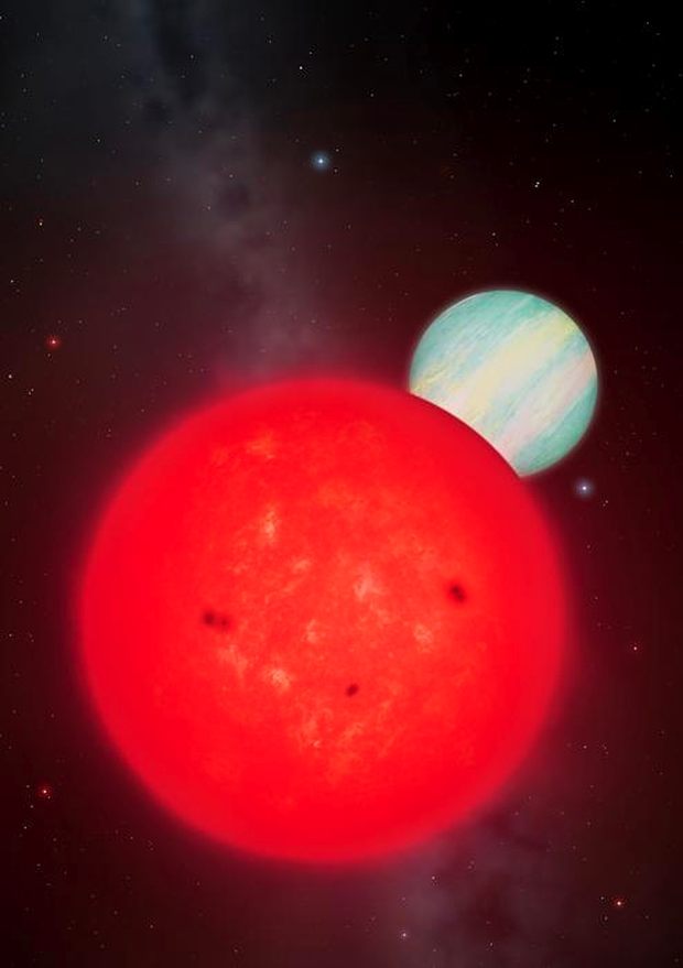
Image: Artwork depicting the exoplanet TOI-6894 b around a red dwarf star. This planet is unusual because, given the size/mass of the planet relative to the very low mass of the star, this planet should not have been able to form. The planet is vary large compared to its parent star, shown here to scale. With the known temperature of the star, the planet is expected to only be approximately 420 degrees Kelvin at the top of its atmosphere. This means its atmosphere may contain methane and ammonia, amongst other species. This would make this planet one of the first planets outside the Solar System where we can observe nitrogen, which alongside carbon and oxygen is a key building block for life. Credit: University of Warwick / Mark Garlick.
TOI-6894 b produces deep transits and sports temperatures in the range of 420 K, according to the study. Clearly this world is not in the ‘hot Jupiter’ category. Amaury Triaud (University of Birmingham) is a co-author on this paper:
“Based on the stellar irradiation of TOI-6894 b, we expect the atmosphere is dominated by methane chemistry, which is exceedingly rare to identify. Temperatures are low enough that atmospheric observations could even show us ammonia, which would be the first time it is found in an exoplanet atmosphere. TOI-6894 b likely presents a benchmark exoplanet for the study of methane-dominated atmospheres and the best ‘laboratory’ to study a planetary atmosphere containing carbon, nitrogen, and oxygen outside the Solar System.”
Thus it’s good to know that JWST observations targeting the atmosphere of this world are already on the calendar within the next 12 months. Rare worlds that can serve as benchmarks for hitherto unexplained processes are pure gold for our investigation of where and how giant planets form.
The paper is Bryant et al., “A transiting giant planet in orbit around a 0.2-solar-mass host star,” Nature Astronomy (2025). Full text. The Kurtovic study is Kurtovic, Pinilla, et al., “Size and Structures of Disks around Very Low Mass Stars in the Taurus Star-Forming Region,” Astronomy & Astrophysics, 645, A139 (2021). Full text.
Expansion of the Universe: An End to the ‘Hubble Tension’?
When one set of data fails to agree with another over the same phenomenon, things can get interesting. It’s in such inconsistencies that interesting new discoveries are sometimes made, and when the inconsistency involves the expansion of the universe, there are plenty of reasons to resolve the problem. Lately the speed of the expansion has been at issue given the discrepancy between measurements of the cosmic microwave background and estimates based on Type Ia supernovae. The result: The so-called Hubble Tension.
It’s worth recalling that it was a century ago that Edwin Hubble measured extragalactic distances by using Cepheid variables in the galaxy NGC 6822. The measurements were necessarily rough because they were complicated by everything from interstellar dust effects to lack of the necessary resolution, so that the Hubble constant was not known to better than a factor of 2. Refinements in instruments tightened up the constant considerably as work progressed over the decades, but the question of how well astronomers had overcome the conflict with the microwave background results remained.

Now we have new work that looks at the rate of expansion using data from the James Webb Space Telescope, doubling the sample of galaxies used to calibrate the supernovae results. The paper’s lead author, Wendy Freedman of the University of Chicago, argues that the JWST results resolve the tension. With Hubble data included in the analysis as well, Freedman calculates a Hubble value of 70.4 kilometers per second per megaparsec, plus or minus 3%. This result brings the supernovae results into statistical agreement with recent cosmic microwave background data showing 67.4, plus or minus 0.7%.
Image: The University of Chicago’s Freedman, a key player in the ongoing debate over the value of the Hubble Constant. Credit: University of Chicago.
While the cosmic microwave background tells us about conditions early in the universe’s expansion, Freedman’s work on supernovae is aimed at pinning down how fast the universe is expanding in the present, which demands accurate measurements of interstellar distances. Knowing the maximum brightness of supernovae allows the use of their apparent luminosities to calculate their distance. Type 1a supernovae are consistent in brightness at their peak, making them, like the Cepheid variables Hubble used, helpful ‘standard candles.’
The same factors that plagued Hubble, such as the effect of dimming from interstellar dust and other factors that affect luminosity, have to be accounted for, but JWST has four times the resolution of the Hubble Space Telescope, and is roughly 10 times as sensitive, making its measurements a new gold standard. Co-author Taylor Hoyt (Lawrence Berkeley Laboratory) notes the result:
“We’re really seeing how fantastic the James Webb Space Telescope is for accurately measuring distances to galaxies. Using its infrared detectors, we can see through dust that has historically plagued accurate measurement of distances, and we can measure with much greater accuracy the brightnesses of stars.”
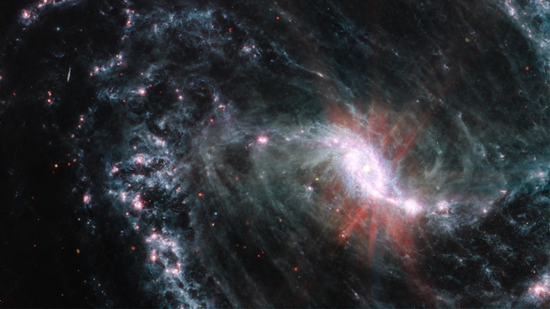
Image: Scientists have made a new calculation of the speed at which the universe is expanding, using the data taken by the powerful new James Webb Space Telescope on multiple galaxies. Above, Webb’s image of one such galaxy, known as NGC 1365. Credit: NASA, ESA, CSA, Janice Lee (NOIRLab), Alyssa Pagan (STScI).
A lack of agreement between the CMB findings and the supernovae data could have been pointing to interesting new physics, but according to this work, the Standard Model of the universe holds up. In a way, that’s too bad for using the discrepancy to probe into mysterious phenomena like dark energy and dark matter, but it seems we’ll have to be looking elsewhere for answers to their origin. Ahead for Freedman and team are new measurements of the Coma cluster that Freedman suggests could fully resolve the matter within years.
As the paper notes:
While our results show consistency with ΛCDM (the Standard Model), continued improvement to the local distance scale is essential for further reducing both systematic and statistical uncertainties.
The paper is Freedman et al., “Status Report on the Chicago-Carnegie Hubble Program (CCHP): Measurement of the Hubble Constant Using the Hubble and James Webb Space Telescopes,” The Astrophysical Journal Vol. 985, No 2 (27 May 2025), 203 (full text).