Centauri Dreams
Imagining and Planning Interstellar Exploration
A Changing Landscape at Ceres
Ceres turns out to be a livelier place than we might have imagined. Continuing analysis of data from the Dawn spacecraft is showing us an object where surface changes evidently caused by temperature variations induced by the dwarf planet’s orbit are readily visible even in short time frames. Two new papers on the Dawn data are now out in Science Advances, suggesting variations in the amount of surface ice as well as newly exposed crustal material.
Andrea Raponi (Institute of Astrophysics and Planetary Science, Rome) led a team that discovered changes at Juling Crater, demonstrating an increase in ice on the northern wall of the 20-kilometer wide crater between April and October of 2016. Calling this ‘the first detection of change on the surface of Ceres,’ Raponi went on to say:
“The combination of Ceres moving closer to the sun in its orbit, along with seasonal change, triggers the release of water vapor from the subsurface, which then condenses on the cold crater wall. This causes an increase in the amount of exposed ice. The warming might also cause landslides on the crater walls that expose fresh ice patches.”
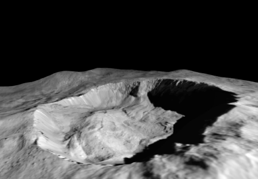
Image: This view from NASA’s Dawn mission shows where ice has been detected in the northern wall of Ceres’ Juling Crater, which is in almost permanent shadow. Dawn acquired the picture with its framing camera on Aug. 30, 2016, and it was processed with the help of NASA Ames Stereo Pipeline (ASP), to estimate the slope of the cliff. Credit: NASA/JPL-Caltech/UCLA/MPS/DLR/IDA/ASI/INAF.
Ceres was moving closer to perihelion in the period following these observations, so we would expect the temperature of areas in shadow to be increasing. Sublimating water ice that had previously accumulated on the cold walls of the crater would be a natural result, and while acknowledging other options — such as falls exposing water ice — the researchers favor a cyclical trend similar to cycles of water ice seen, for example, at Comet 67P/Churyumov-Gerasimenko. From the paper:
The linear relationship between ice abundance and solar flux… supports the possibility of solar flux as the main factor responsible for the observed increase. The water ice abundance on the wall is probably not constantly increasing over a longer time range. More likely, we are observing only part of a seasonal cycle of water sublimation and condensation, in which the observed increase should be followed by a decrease.
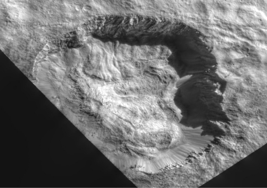
Image: This view from NASA’s Dawn mission shows the floor of Ceres’ Juling Crater. The crater floor shows evidence of the flow of ice and rock, similar to rock glaciers in Earth’s polar regions. Dawn acquired the picture with its framing camera on Aug. 30, 2016. Credit: NASA/JPL-Caltech/UCLA/MPS/DLR/IDA/ASI/INAF.
A short-term variation in surface water ice shows us an active body, a result that meshes with further observations from Dawn’s visible and infrared mapping spectrometer (VIR) showing variability in Ceres’ crust and the likelihood of newly exposed material. The work, led by Giacomo Carrozzo of the Institute of Astrophysics and Planetary Science, identifies twelve sites rich in sodium carbonates and takes a tight look at several areas where water is present as part of the carbonate structure.
Although carbonates had previously been found on Ceres, this is the first identification of hydrated carbonate there. The fact that water ice is not stable over long time periods on the surface of Ceres unless hidden in shadow, and that hydrated carbonate would dehydrate over timescales of a few million years, means that these sites have been exposed, says Carrozzo, to recent activity on the surface.

Image: This view from NASA’s Dawn mission shows Ceres’ tallest mountain, Ahuna Mons, 4 kilometers high and 17 kilometers wide. This is one of the few sites on Ceres at which a significant amount of sodium carbonate has been found, shown in green and red colors in the lower right image. The top and lower left images were collected by Dawn’s framing camera. The top image is a 3D view reconstructed with the help of topography data. Credit: NASA/JPL-Caltech/UCLA/MPS/DLR/IDA/ASI/INA.
Taken together, the water ice findings and the presence of hydrated sodium carbonates speak to the geological and chemical activity that continues on Ceres. As the paper notes:
The different chemical forms of the sodium carbonate, their fresh appearance, morphological settings, and the uneven distribution on Ceres indicate that the formation, exposure, dehydration, and destruction processes of carbonates are recurrent and continuous in recent geological time, implying a still-evolving body and modern processes involving fluid water.
The papers are Carrozzo et al., “Nature, formation, and distribution of carbonates on Ceres,” Science Advances Vol. 4, No. 3 (14 March 2018) e1701645 (abstract); and Raponi et al., “Variations in the amount of water ice on Ceres’ surface suggest a seasonal water cycle,” Science Advances Vol. 4, No. 2 (14 March 2018) eaao3757 (abstract).

Red Dwarfs: Their Impact on Biosignatures
We’re in the midst of a significant period defining the biosignatures life can produce and determining how we might identify them. Centauri Dreams regular Alex Tolley today looks at a paper offering a unique contribution to this effort. The work of Sarah Rugheimer and Lisa Kaltenegger, the paper looks at how exoplanet spectra change for different types of host star and different epochs of planetary evolution. As Alex points out, the effects are profound, especially given the fact that red dwarfs will be our testbed for biosignature detection as we probe planetary atmospheres during transits around nearby stars. How stellar class affects our analysis will affect our strategies especially as we probe early Earth atmosphere equivalents. What will we find, for example, at TRAPPIST-1?
By Alex Tolley

As the search for life on exoplanets ramps up, the question arises as to which types of stars represent the best targets. Based on distribution, M-Dwarfs are very attractive as they represent 3/4 of all stars in our galaxy. Their long lifetimes offer abundant opportunities for life to evolve, and to resist extinction as their stars increase in luminosity. On Earth, terrestrial life might last another one billion years before the level of CO2 in the atmosphere is forced to be reduced below photosynthetic requirements for plants to survive. All but lithophilic life might be extinct within 1 ½ billion years. An additional advantage for astronomers is that spectra of exoplanet atmospheres will be easier to distinguish around low luminosity stars. [6, 7]
From a purely numbers game, M-Dwarfs are most attractive targets:
“Temperate terrestrial planets transiting M-dwarf stars are often touted as the poor-astronomer’s Earth analog, since they are easier to detect and characterize than a true Earth twin. Based on what we currently know, however, M-Dwarf planets are the most common habitable worlds“ [1]

Image: Gliese 581 from a planet in its HZ. Credit: David Hardy.
That M-Dwarf rocky worlds may be the most common habitable world is due to:
“1. rocky planets are much more common in the temperate zones of M-Dwarfs (…) than in the temperate zones of Sun-like Stars (…)
2. small stars are more common than big stars (…)
3. the tidally-locked nature of these planets is not a challenge to climate and may double the width of the habitable zone (…)
4. the red stellar radiation results in a weaker ice-albedo feedback
and hence stabler climate (…), and (…)5. the slow main sequence evolution of M-Dwarfs means that a geological thermostat is not strictly necessary to maintain habitable conditions for billions of years (…). Studying temperate terrestrial planets around M-Dwarfs is our best shot at understanding habitability writ large.” [1]
There are negatives for life around M-Dwarfs too. The closeness of the habitable zone (HZ) to the star results in tidal locking that may impact the stability of the atmosphere, as well as the intense flares that may strip the atmospheres from these worlds. However, these negatives for habitability and hence life may be compensated by the ubiquity of such worlds and the relative ease of studying them remotely. For lithophilic life, surface conditions largely can be ignored.
After the lifeless Hadean, the Archean and Proterozoic eons had life that was purely prokaryotic. During this time photosynthesis evolved that eventually resulted in an atmosphere with O2 and very little CO2 and CH4. This phase of life’s history covers the long period when Earth’s atmosphere changed from a largely reducing one of N2, CO2, and some CH4, to one that becomes oxidizing. The Phanerozoic, starting around 500 mya encompasses the period when O2 pressures increased to the level they are today and terrestrial, multicellular life blossomed in diversity.
If Earth’s history is any guide, life in our galaxy will be mostly unicellular bacteria, living in a reducing atmosphere. If that is a correct hypothesis, then most life in the galaxy will be non-photosynthetic, perhaps with biologies similar to the Archaea. A biosignature of such microbial life will still require looking for a disequilibrium in gases, mainly CO2 and CH4, rather than O2 and CH4 [2, 3]. Archaea include the extremophiles living in a diverse array of environments, including the lithosphere. Such organisms may well survive the harsher conditions of a tidally locked world, especially regarding the impact of flares.
The question then arises, if we look for a biosignature around stars of different spectral types, will the star’s type have an impact on the planet’s atmosphere, detectable spectral markers, and any potential biosignatures?
This question is examined in a paper by Rugheimer and Kaltenegger [5]. The authors modeled the spectra of atmospheres to simulate Earth-like worlds – rocky worlds large enough to hold an atmosphere and presumably with a mix of ocean and continents, rather than water worlds – orbiting in the HZ of different star types F, G, K and M. Their simulations cover the state of evolution of those worlds as if they were an Earth relocated to other stars, so that the spectra for different gas mixtures could be modeled.
The light of an M-Dwarf is shifted so that the UV component is much diminished. This affects the reactions of the gases in the atmosphere. Photolysis is reduced, reducing the loss of H20, which in turn, as a greenhouse gas, warms the surface more than with a hotter star. CH4 in particular is not lost and may even result in a runaway accumulation in some cases. The increase in H2O increases the cloud cover in the troposphere, which in turn increases the planet’s albedo. The increased IR component of the M-Dwarf’s output increases the surface temperature as well and may well further increase cloud formation.
The photolysis of water and the oxidation of CH4 is shown below. UV is required which results in the reduced loss of H2O and CH4 on exoplanets around M-Dwarfs.
H2O + hv (? < 200 nm) -> H + OH
CH4 + OH -> CH3 + H2O
Similarly, UV is required to split O2 allowing O3 formation.
O2 + hv (? < 240 nm) -> O + O
O + O2 -> O3
Previously, Kaltenegger [4] had modeled the atmospheres of Earth-like worlds around different stars and constructed synthetic spectra to determine the visibility of different biosignature gases in the visible and near-infrared.
Following on, Rugenheimer et al modeled gases for 4 different periods – 3.9, 2.0, 0.8 and 0 Ga for the 4 star types. The initial gas mixes are shown in Table 1.
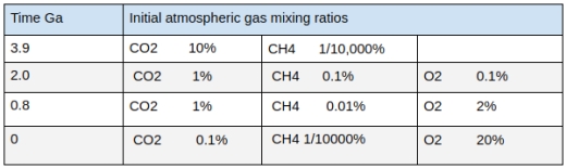
Table1. Gas mixing ratios for 4 eons. N2 not shown.
Because the stars age at different rates, the periods are standardized to Earth. As M-Dwarfs age far more slowly than our sun, the different luminosities are modeled as if their planets are further out from their star earlier in its history to simulate the lower luminosity.
The result of the simulations shows that some markers will be difficult to observe under different spectral types of stars.
The impact of the star type is shown in Figure 1. Temperature and 5 gases are profiled with altitude, The M-Dwarfs show clear differences from the hotter star types. Of particular note are the higher H2O and CH4 atmosphere ratios, particularly at higher altitudes.
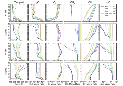
Figure 1. Planetary temperature vs. altitude profiles and mixing ratio profiles for H2O, O3, CH4, OH, and N2O (left to right) for a planet orbiting the grid of FGKM stellar models with a prebiotic atmosphere corresponding to 3.9 Ga (first row), the early rise of oxygen at 2.0 Ga (second row), the start of multicellular life on Earth at 0.8 Ga (third row), and the modern atmosphere (fourth row). Source: Rugheimer & Kaltenegger 2017 [5]
Figure 2 shows the simulated spectra for the star types. Because of the loss of shorter wavelengths with M-Dwarf stars, the O2 signatures are largely lost. This means that even should a planet around an M-Dwarf evolve photosynthesis and create an oxidizing atmosphere, this may not be detectable around such a world.
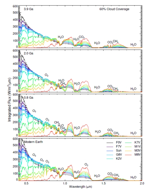
Figure 2. Disk-integrated VIS/NIR spectra at a resolution of 800 at the TOA for an Earth-like planet for the grid of stellar and geological epoch models assuming 60% Earth-analogue cloud coverage. For individual features highlighting the O2, O3, and H2O/CH4 bands in the VIS spectrum. Source: Rugheimer & Kaltenegger 2017 [5] [TOA = Top of the atmosphere – AMT]
In contrast, the strong markers for CO2 and CH4 are well represented in the spectrum for M type stars. This creates a complication for a biosignature for early life comparable to the Archean and early Proterozoic periods on Earth. An atmosphere of CO2 and CH4 assumes that the CH4 is due to methanogens being the dominant source of CH4, far outstripping geologic sources. On the Hadean Earth, CH4 outgassing should be rapidly eliminated by UV. During the Archean, the biogenic production of CH4 maintains the CH4 and therefore the disequilibrium biosignature. But on an M-Dwarf world, this CH4 photolysis is largely absent, resulting in a CO2/CH4 biosignature that is a false positive.
If photosynthesis evolves, the O2 signal can be detected at the longer wavelength of 760 nm, but only if there is no cloud cover, as shown in figure 3. For an M-Dwarf planet, clouds mask the O2 signal, and we expect more cloud cover due to the increased H2O on such worlds.
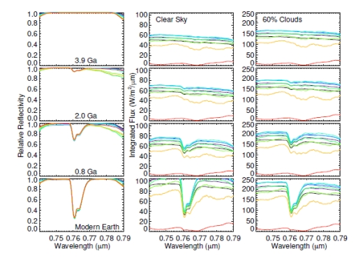
Figure 3. Disk-integrated spectra (R = 800) of the O2 feature at 0.76 m for clear sky in relative reflectivity (left) and the detectable reflected emergent flux for clear sky (middle) and 60% cloud cover (right). Source: Rugheimer & Kaltenegger 2017 [5]. Note the loss of detectable O2 feature for M-type stars – AMT
Fortunately, ozone (O3) can be detected strongly in the IR around 9500 nm, so we can hope to detect photosynthetic life when the O2 partial pressure increases. Figure 4 shows that the O3 signature can be detected in the Archean in the Phanerozoic, but not the Proterozoic.
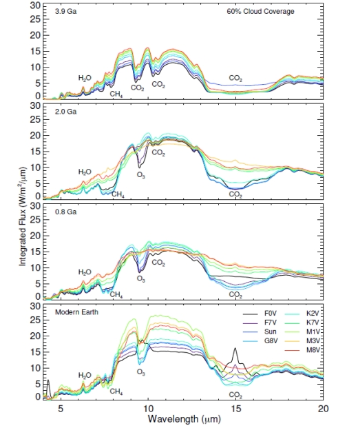
Figure 4. Smoothed, disk-integrated IR spectra at the TOA for an Earth-like planet for the grid of stellar and geological epoch models assuming 60% Earth-analogue cloud coverage. For individual features highlighting the O3, H2O/CH4, and CO2 bands in the IR spectrum see Figs. 9, 10, and 11, respectively. Source: Rugheimer & Kaltenegger 2017 [5]
While current instruments cannot resolve spectra in sufficient detail to detect the needed signatures of gases, the authors conclude
“These spectra can be a useful input to design instruments and to optimize the observation strategy for direct imaging or secondary eclipse observations with EELT or JWST as well as other future mission design concepts such as LUVOIR/HDST.”
To conclude, the type of star complicates biosignature detection, especially the co-presence of CO2 and CH4 in Archean and early Proterozoic eons that dominate the history of life on Earth. Not only is the star’s light shifted, hiding shorter wavelength signals, but the light itself impacts the equilibrium composition of atmospheric gases which can lead to biosignature ambiguity.
While the ubiquity of M-Dwarf stars and the longevity of low O2 atmospheres due to the time to evolve photosynthesis on Earth and the delay before the atmosphere builds up its O2 partial pressure, favors M-Dwarf stars as targets for looking for early life, the potential of false positives for the Archaean and early Proterozoic equivalent eons complicates the search for life on these worlds using expected biosignatures for worlds around sol-like stars. There is still work to be done to resolve these issues.
References
1. N. B. Cowan et al “Characterizing Transiting Planet Atmospheres through 2025”
2015 PASP 127 311. DOI: https://doi.org/10.1086/680855
2. Tolley, A, “Detecting Early Life on Exoplanets”, 02/23/2018. https://centauri-dreams.org/2018/02/23/detecting-early-life-on-exoplanets/
3. Krissansen-Totton et al “Disequilibrium biosignatures over Earth history and implications for detecting exoplanet life” 2018 Science Advances Vol. 4, no. 1. DOI: 10.1126/sciadv.aao5747
4. Kaltenegger et al “Spectral Evolution of an Earth-like Planet”, The Astrophysical Journal, 658:598Y616, 2007 March 20 (abstract).
5. Rugheimer, Kaltenegger “Spectra of Earth-like Planets Through Geological Evolution Around FGKM Stars”, The Astrophysical Journal 854(1). DOI: 10.3847/1538-4357/aaa47a
6. Burrows, A. S ”Spectra as windows into exoplanet atmospheres,” 2014, PNAS, 111, 12601 (abstract)
7. Ehrenreich D “Transmission spectra of exoplanet atmospheres” 2011 http://www-astro.physik.tu-berlin.de/plato-2011/talks/PLATO_SC2011_S03T06_Ehrenreich.pdf
Maxing Out Kepler
What happens to a spacecraft at the end of its mission depends on where it’s located. We sent Galileo into Jupiter on September 21, 2003 not so much to gather data but because the spacecraft had not been sterilized before launch. A crash into one of the Galilean moons could potentially have compromised our future searches for life there, but a plunge into Jupiter’s atmosphere eliminated the problem.
Cassini met a similar fate at Saturn, and in both cases, the need to keep a fuel reserve available for that final maneuver was paramount. Now we face a different kind of problem with Kepler, a doughty spacecraft that has more than lived up to its promise despite numerous setbacks, but one that is getting perilously low on fuel. With no nearby world to compromise, Kepler’s challenge is to keep enough fuel in reserve to maximize its scientific potential before its thrusters fail, thus making it impossible for the spacecraft to be aimed at Earth for data transfer.
In an Earth-trailing orbit 151 million kilometers from Earth, Kepler’s fuel tank is expected to run dry within a few months, according to this news release from NASA Ames. The balancing act for its final observing run will be to reserve as much fuel as needed to aim the spacecraft, while gathering as much data as possible before the final maneuver takes place. Timing this will involve keeping a close eye on the fuel tank’s pressure and the performance of the Kepler thrusters, looking for signs that the end is near.
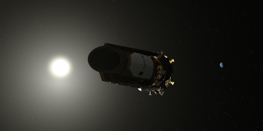
Image: K2 at work, in this image from NASA Ames.
Meanwhile, as we await the April launch of the Transiting Exoplanet Survey Satellite (TESS), we can reflect on Kepler’s longevity. The failure of its second reaction wheel ended the primary mission in 2013, but as we’ve discussed here on many occasions, the use of photon momentum to maintain its pointing meant that the craft could be reborn as K2, an extended mission that shifted its field of view to different portions of the sky on a roughly three-month basis.
As the mission team had assumed that Kepler was capable of about 10 of these observing campaigns, the fact that the mission is now on its 17th is another Kepler surprise. The current campaign, entered this month, will presumably be its last, but if we’ve learned anything about this spacecraft, it’s that we shouldn’t count it out. Let’s see how long the fuel will last.
Antimatter: The Heat Problem

My family has had a closer call with ALS than I would ever have wished for, so the news of Stephen Hawking’s death stays with me as I write this morning. I want to finish up my thoughts on antimatter from the last few days, but I have to preface that by noting how stunning Hawking’s non-scientific accomplishment was. In my family’s case, the ALS diagnosis turned out to be mistaken, but there was no doubt about Hawking’s affliction. How on Earth did he live so long with an illness that should have taken him mere years after it was identified?
Hawking’s name will, of course, continue to resonate in these pages — he was simply too major a figure not to be a continuing part of our discussions. With that in mind, and in a ruminative mood anyway, let me turn back to the 1950s, as I did yesterday in our look at Eugen Sänger’s attempt to create the design for an antimatter rocket. Because even as Sänger labored over the idea, one he had been pursuing since the 1930s, Les Shepherd was looking at the antimatter prospect, and coming up with aspects of the problem not previously identified.
Getting a Starship Up to Speed
Shepherd isn’t as well known as he should be to the public, but within the aerospace community he is something of a legend. A specialist in nuclear fusion, his activities within the International Academy of Astronautics (he was a founder) and the International Astronautical Federation (he was its president) were legion, but this morning I turn to “Interstellar Flight,” a Shepherd paper from 1952. This was published just a year before Sänger explained his antimatter rocket ideas to the 4th International Astronautical Congress in Zurich, later published in Space-Flight Problems (1953).

Remember that neither of these scientists knew about the antiproton as anything other than a theoretical construct, which meant that a ‘photon rocket’ in the Sänger mode just wasn’t going to work. But Shepherd saw that even if it could be made to function, antimatter propulsion ran into other difficulties. Producing and storing antimatter were known problems even then, but it was Shepherd who saw that “The most serious factor restricting journeys to the stars, indeed, is not likely to be the limitation on velocity but rather limitation on acceleration.”
This stems from the fact that the matter/antimatter annihilation is so mind-bogglingly powerful. Let me quote Shepherd on this, as the problem is serious:
…a photon rocket accelerating at 1 g would require to dissipate power in the exhaust beam at the fantastic rate of 3 million Megawatts/tonne. If we suppose that the photons take the form of black-body radiation and that there is 1 sq metre of radiating surface available per tonne of vehicle mass then we can obtain the necessary surface temperature from the Stefan-Boltzmann law…
Shepherd worked this out as:
5.7 x 10⁻⁸ T4 = 3 x 10¹² watts/metre2
with T expressed in degrees Kelvin. So the crux of the problem is that we are producing an emitting surface with a temperature in the range of 100,000 K. The problem with huge temperatures is that we have to find some way of dissipating them. We’d like to get our rocket operating at 1 g acceleration so we could tour the galaxy, using relativistic time dilation to send a crew to the galactic center, for example, within a human lifetime. But we have to dispose of waste heat from the extraordinarily hot emitting surfaces of our spacecraft, because with numbers like these, even the most efficient engine is still going to produce waste heat.

Image: What I liked about the ‘Venture Star’ from James Cameron’s film Avatar was that the design included radiators, clearly visible in this image. How often have we seen the heat problem addressed in any Hollywood offering? Nice work.
Now we can look at Robert Frisbee’s design — an antimatter ‘beamed-core’ starship forced by its nature to be thousands of kilometers long and, compared to its length, incredibly thin. Frisbee’s craft assumes, as I mentioned, a beamed-core design, with pions from the annihilation of protons and antiprotons being shaped into a stream of thrust by a magnetic nozzle; i.e., a superconducting magnet. The spacecraft has to be protected against the gamma rays produced in the annihilation process and it needs radiators to bleed off all the heat generated by the engine.
We also need system radiators for the refrigeration systems. Never forget that we’re storing antimatter within a fraction of a degree of absolute zero (-273 C), then levitating it using a magnetic field that takes advantage of the paramagnetism of frozen hydrogen. Thus:
…the width of the main radiator is fixed by the diameter of the superconductor magnet loop. This results in a very long main radiator (e.g., hundreds of km in length), but it does serve to minimize the radiation and dust shields by keeping the overall vehicle long and thin.
Frisbee wryly notes the need to consider the propellant feed in systems like this. After all, we’re trying to send antimatter pellets magnetically down a tube at least hundreds of kilometers long. The pellets are frozen at 1 K, but we’re doing this in an environment where our propellant feed is sitting next to a 1500 K radiator! Frisbee tries to get around this by converting the anti-hydrogen into antiprotons, feeding these down to the engine in the form of a particle beam.
Frisbee’s 40 light-year mission with a duration of 100 years is set up as a four-stage antimatter rocket massing millions of tons, with radiator length for the first stage climbing as high as 7500 kilometers, and computed radiator lengths for the later stages still in the hundreds of kilometers. Frisbee points out that the 123,000 TW of first-stage engine ‘jet’ power demands the dumping of 207,000 TW of 200 MeV gamma rays. Radiator technology will need an extreme upgrade.
And to drop just briefly back to antimatter production, check this out:
The full 4-stage vehicle requires a total antiproton propellant load of 39,300,000 MT. The annihilation (MC2) energy of this much antimatter (plus an equal amount of matter) corresponds to ~17.7 million years of current Human energy output. At current production efficiencies (10-9), the energy required to produce the antiprotons corresponds to ~17.7 quadrillion [1015] years of current Human energy output. For comparison, this is “only” 590 years of the total energy output of sun. Even at the maximum predicted energy efficiency of antiproton production (0.01%), we would need 177 billion years of current Human energy output for production. In terms of production rate, we only need about 4×10²¹ times the current annual antiproton production rate.
Impossible to build, I’m sure. But papers like these are immensely useful. They illustrate the consequences of taking known theory into the realm of engineering to see what is demanded. We need to know where the showstoppers are to continue exploring, hoping that at some point we find ways to mitigate them. Frisbee’s paper is available online, and repays a close reading. We could use the mind of a future Hawking to attack such intractable problems.
The Les Shepherd paper cited above is “Interstellar Flight,” JBIS, Vol. 11, 149-167, July 1952. The Frisbee paper is “How to Build an Antimatter Rocket for Interstellar Missions,” 39th AIAA/ASME/SAE/ASEE Joint Propulsion Conference and Exhibit, 20-23 July 2003 (full text).
Stephen Hawking (1942-2018)
The Tau Zero Foundation expresses it deepest sympathies to the family, friends and colleagues of Stephen Hawking. His death is a loss to the the world, to our scientific communities, and to all who value courage in the face of extreme odds.
Harnessing Antimatter for Propulsion
Antimatter’s staggering energy potential always catches the eye, as I mentioned in yesterday’s post. The problem is how to harness it. Eugen Sänger’s ‘photon rocket’ was an attempt to do just that, but the concept was flawed because when he was developing it early in the 1950s, the only form of antimatter known was the positron, the antimatter equivalent of the electron. The antiproton would not be confirmed until 1955. A Sänger photon rocket would rely on the annihilation of positrons and electrons, and therein lies a problem.

Sänger wanted to jack up his rocket’s exhaust velocity to the speed of light, creating a specific impulse of a mind-boggling 3 X 10⁷ seconds. Specific impulse is a broad measure of engine efficiency, so that the higher the specific impulse, the more thrust for a given amount of propellant. Antimatter annihilation could create the exhaust velocity he needed by producing gamma rays, but positron/electron annihilation was essentially a gamma ray bomb, pumping out gamma rays in random directions.
Image: Austrian rocket scientist Eugen Sänger, whose early work on antimatter rockets identified the problems with positron/electron annihilation for propulsion.
What Sänger needed was thrust. His idea of an ‘electron gas’ to channel the gamma rays his photon rocket would produce never bore fruit; in fact, Adam Crowl has pointed out in these pages that the 0.511 MeV gamma rays generated in the antimatter annihilation would demand an electron gas involving densities seen only in white dwarf stars (see Re-thinking the Antimatter Rocket). No wonder Sänger was forced to abandon the idea.
The discovery of the antiproton opened up a different range of possibilities. When protons and antiprotons annihilate each other, they produce gamma rays and, usefully, particles called pi-mesons, or pions. I’m drawing on Greg Matloff’s The Starflight Handbook (Wiley, 1989) in citing the breakdown: Each proton/antiproton annihilation produces an average of 1.5 positively charged pions, 1.5 negatively charged pions and 2 neutral pions.
Note the charge. We can use this to deflect some of these pions, because while the neutral ones decay quickly, the charged pions take a bit longer before they decay into gamma rays and neutrinos. In this interval, Robert Forward saw, we can use a magnetic nozzle created through superconducting coils to shape a charged pion exhaust stream. The charged pions will decay, but by the time they do, they will be far behind the rocket. We thus have useful momentum from this fleeting interaction or, as Matloff points out, we could also use the pions to heat an inert propellant — hydrogen, water, methane — to produce a channeled thrust.

But while we now have a theoretical way to produce thrust with an antimatter reaction, we still have nowhere near the specific impulse Sänger hoped for, because our ‘beamed core’ antimatter rocket can’t harness all the neutral pions produced by the matter/antimatter annihilation. My friend Giovanni Vulpetti analyzed the problem in the 1980s, concluding that we can expect a pion rocket to achieve a specific impulse equivalent to 0.58c. He summed the matter up in a paper in the Journal of the British Interplanetary Society in 1999:
In the case of proton-antiproton, annihilation generates photons, massive leptons and mesons that decay by chain; some of their final products are neutrinos. In addition, a considerable fraction of the high-energy photons cannot be utilised as jet energy. Both carry off about one third of the initial hadronic mass. Thus, it is not possible to control such amount of energy.
Image: Italian physicist Giovanni Vulpetti, a major figure in antimatter studies through papers in Acta Astronautica, JBIS and elsewhere.
We’re also plagued by inefficiencies in the magnetic nozzle, a further limitation on exhaust velocity. But we do have, in the pion rocket, a way to produce thrust if we can get around antimatter’s other problems.
In the comments to yesterday’s post, several readers asked about creating anti-hydrogen (a positron orbiting an antiproton), a feat that has already been accomplished at CERN. In fact, Gerald Jackson and Steve Howe (Hbar Technologies) created an unusual storage solution for anti-hydrogen in their ‘antimatter sail’ concept for NIAC, which you can see described in their final NIAC report. In more recent work, Jackson has suggested the possibility of using anti-lithium rather than anti-hydrogen.
The idea is to store the frozen anti-hydrogen in a chip much like the integrated circuit chips we use every day in our electronic devices. A series of tunnels on the chip (think of the etching techniques we already use with electronics) lead to periodic wells where the anti-hydrogen pellets are stored, with voltage changes moving them from one well to another. The anti-hydrogen storage bottle draws on methods Robert Millikan and Harvey Fletcher used in the early 20th Century to measure the charge of the electron to produce a portable storage device.
The paramagnetism of frozen anti-hydrogen makes this possible, paramagnetism being the weak attraction of certain materials to an externally applied magnetic field. Innovative approaches like these are changing the way we look at antimatter storage. Let me quote Adam Crowl, from the Centauri Dreams essay I cited earlier:
The old concept of storing [antimatter] as plasma is presently seen as too power intensive and too low in density. Newer understanding of the stability of frozen hydrogen and its paramagnetic properties has led to the concept of magnetically levitating snowballs of anti-hydrogen at the phenomenally low 0.01 K. This should mean a near-zero vapour pressure and minimal loses to annihilation of the frozen antimatter.
But out of this comes work like that of JPL’s Robert Frisbee, who has produced an antimatter rocket design that is thousands of kilometers long, the result of the need to store antimatter as well as to maximize the surface area of the radiators needed to keep the craft functional. In Frisbee’s craft, antimatter is stored within a fraction of a degree of absolute zero (-273 C) and then levitated in a magnetic field. Imagine the refrigeration demands on the spacecraft in sustaining antimatter storage while also incorporating radiators to channel off waste heat.
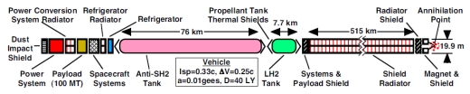
Image: An antimatter rocket as examined by Robert Frisbee. This is Figure 6 from the paper cited below. Caption: Conceptual Systems for an Antimatter Propulsion System.
Radiators? I’m running out of space this morning, so we’ll return to antimatter tomorrow, when I want to acknowledge Les Shepherd’s early contributions to the antimatter rocket concept.
The paper by Giovanni Vulpetti I quoted above is “Problems and Perspectives in Interstellar Exploration,” JBIS Vol. 52, No. 9/10, available on Vulpetti’s website. For Frisbee’s work, see for example “How to Build an Antimatter Rocket for Interstellar Missions,” 39th AIAA/ASME/SAE/ASEE Joint Propulsion Conference and Exhibit, 20-23 July 2003 (full text).

Follow with RSS or E-Mail
