Centauri Dreams
Imagining and Planning Interstellar Exploration
Assembly theory (AT) – A New Approach to Detecting Extraterrestrial Life Unrecognizable by Present Technologies
With landers on places like Enceladus conceivable in the not distant future, how we might recognize extraterrestrial life if and when we run into it is no small matter. But maybe we can draw conclusions by addressing the complexity of an object, calculating what it would take to produce it. Don Wilkins considers this approach in today’s essay as he lays out the background of Assembly Theory. A retired aerospace engineer with thirty-five years experience in designing, developing, testing, manufacturing and deploying avionics, Don tells me he has been an avid supporter of space flight and exploration all the way back to the days of Project Mercury. Based in St. Louis, where he is an adjunct instructor of electronics at Washington University, Don holds twelve patents and is involved with the university’s efforts at increasing participation in science, technology, engineering, and math. Have a look at how we might deploy AT methods not only in our system but around other stars.
by Don Wilkins
A continuing concern within the astrobiology community is the possibility alien life is detected, then misclassified as built from non-organic processes. Likely harbors for extraterrestrial life — if such life exists — might be so alien, employing chemistries radically different from those used by terrestrial life, as to be unrecognizable by present technologies. No definitive signature unambiguously distinguishes life from inorganic processes. [1]
Two contentious results from the search for life on Mars are examples of this uncertainty. Lack of knowledge of the environments producing the results prevented elimination of abiotic origins for the molecules under evaluation. The Viking Lander’s metabolic experiments provide debatable results as the properties of Martian soil were unknown. An exciting announcement of life detection in the ALH 84001 meteorite is challenged as the ambiguous criteria to make the decision are not quantitative.
Terrestrial living systems employ processes such as photosynthesis, whose outputs are potential biosignatures. While these signals are relatively simple to identify on Earth, the unknown context of these signals in alien environments makes distinguishing between organic and inorganic origins difficult if not impossible.
The central problem arises in an apparent disconnect between physics and biology. In accounting for life, traditional physics provides the laws of nature, and assumes specific outcomes are the result of specific initial conditions. Life, in the standard interpretation, is encoded in the initial period immediately after the Big Bang. Life is, in other words, an emergent property of the Universe.
Assembly theory (AT) offers a possible solution to the ambiguity. AT posits a numerical value, based on the complexity of a molecule, that can be assigned to a chemical, the Assembly Index (AI), Figure 1. This parameter measures the histories of an object, essentially the complexity of the processes which formed the molecule. Assembly pathways are sequences of joining operations, from basic building blocks to final product. In these sequences, sub-units generated within the sequence combine with other basic or compound sub-units later in the sequence, to recursively generate larger structures. [2]
The theory purports to objectively measure an object’s complexity by considering how it was made. The assembly index (AI) is produced by calculating the minimum number of steps needed to make the object from its ingredients. The results showed, for relatively small molecules (mass?<?~250 Daltons), AI is approximately proportional to molecular weight. The relationship with molecular weight is not valid for large molecules greater than 250 Daltons. Note: One Dalton or atomic mass unit is a equal to one twelfth of the mass of a free carbon-12 atom at rest.
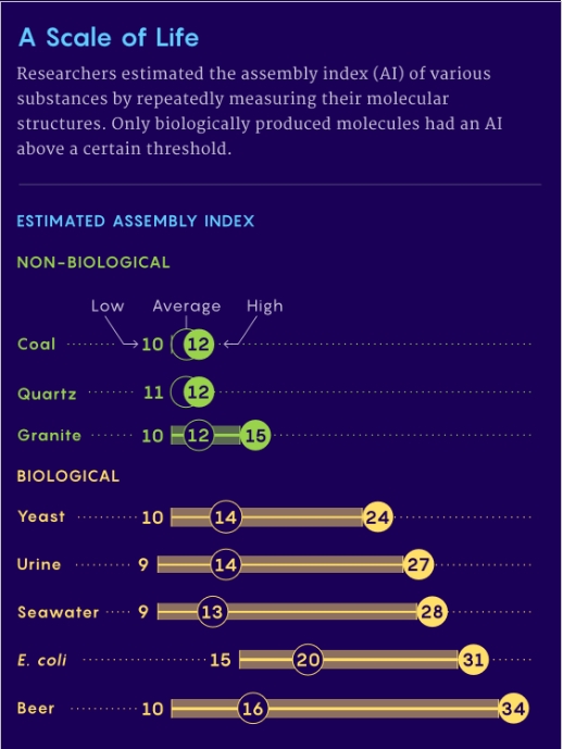
Figure 1. A Comparison of Assembly Indices for Biological and Abiotic Molecules.
Analyzing a molecule begins with basic building blocks, a shared set of objects, Figure 2. AI measures the smallest number of joining operations required to create the object. The assembly process is a random walk on weighted trees where the number of outgoing edges (leaves) grows as a function of the depth of the tree. A probability estimate an object forms by chance requires the production of several million trees and calculating the likelihood of the most likely path through the “forest”. Probability is related to the number of joining operations required or the path length traversed to produce the molecule. As an example, the probability of Taxol forming ranges between 1:1035 to 1:1060 with a path length of 30. In Figure 2, alpha biasing controls how quickly the number of joining operations grows with the depth of the tree.

Figure 2. Calculating Complexity
AT does not require extremely fine-tuned initial conditions demanded in the physics-based origins of life. Information to build specific objects accumulates over time. A highly improbable fine-tuned Big Bang is no longer needed. AT takes advantage of concepts borrowed from graph (networks of interlinked nodes) theory. [3] According to Sara Walker of Arizona State University and a lead AT researcher, information “is in the path, not the initial conditions.”
To explain why some objects appear but others do not, AT posits four distinct classifications, Figure 3. All possible basic building block variations are allowed in the Assembly Universe. Physics, temperature or catalysis are examples, constraining the combinations, eliminating constructs which are not physical in the Assembly Possible. Only objects that can be assembled comprise the Assembly Contingent level. Observable objects are grouped in the Assembly Observed.

Figure 3. The four “universes” of Assembly Theory
Chiara Marletto, a theoretical physicist at the University of Oxford, with David Deutsch, a physicist also at Oxford, are developing a theory resembling AT, the constructor theory (CT). Mimicking the thermodynamics Carnot cycle, CT uses machines or constructors operating in a cyclic fashion, starting at a original state, processing through a pattern until the process returns to the original state to explain a non-probabilistic Universe.
A team headed by Lee Cronin of the University of Glasgow and Sara Walker proposes AT as a tool to distinguish between molecules produced by terrestrial or extraterrestrial life and those built by abiotic processes. [4] AT analysis is susceptible to false negatives but current work produces no false positives. After completing a series of demonstrations, the researchers believe an AT life detection experiment deployable to extraterrestrial locations is possible.
Researchers believe AI estimates can be made using mass or infrared spectrometry. [5-6] While mass spectrometry requires physical access to samples, Cronin and colleagues showed a combination of AT and infrared spectrometry sensors similar to those on the James Webb Space Telescope could analyze the chemical environment of an exoplanet, possibly detecting alien life.
References
[1] Philip Ball, A New Idea for How to Assemble Life, Quanta, 4 May 2023,
https://www.quantamagazine.org/a-new-theory-for-the-assembly-of-life-in-the-universe-20230504?mc_cid=088ea6be73&mc_eid=34716a7dd8
[2] Abhishek Sharma, Dániel Czégel, Michael Lachmann, Christopher P. Kempes, Sara I. Walker, Leroy Cronin, “Assembly Theory Explains and Quantifies the Emergence of Selection and Evolution,”
https://arxiv.org/abs/2206.02279
[3] Stuart M. Marshall, Douglas G. Moore, Alastair R. G. Murray, Sara I. Walker, and Leroy Cronin, Formalising the Pathways to Life Using Assembly Spaces, Entropy 2022, 24(7), 884, 27 June 2022, https://doi.org/10.3390/e24070884
[4] Yu Liu, Cole Mathis, Micha? Dariusz Bajczyk, Stuart M. Marshall, Liam Wilbraham, Leroy Cronin, “Ring and mapping chemical space with molecular assembly trees,” Science Advances, Vol. 7, No. 39
https://www.science.org/doi/10.1126/sciadv.abj2465
[5] Stuart M. Marshall, Cole Mathis, Emma Carrick, Graham Keenan, Geoffrey J. T. Cooper, Heather Graham, Matthew Craven, Piotr S. Gromski, Douglas G. Moore, Sara I. Walker, Leroy Cronin, “Identifying molecules as biosignatures with assembly theory and mass spectrometry,” Nature Communications volume 12, article number: 3033 (2021)
https://www.nature.com/articles/s41467-021-23258-x
[6] Michael Jirasek, Abhishek Sharma, Jessica R. Bame, Nicola Bell1, Stuart M. Marshall,Cole Mathis, Alasdair Macleod, Geoffrey J. T. Cooper!, Marcel Swart, Rosa Mollfulleda, Leroy Cronin, “Multimodal Techniques for Detecting Alien Life using Assembly Theory and Spectroscopy,” https://arxiv.org/ftp/arxiv/papers/2302/2302.13753.pdf

Game Changer: Exploring the New Paradigm for Deep Space
The game changer for space exploration in coming decades will be self-assembly, enabling the growth of a new and invigorating paradigm in which multiple smallsat sailcraft launched as ‘rideshare’ payloads augment huge ‘flagship’ missions. Self-assembly allows formation-flying smallsats to emerge enroute as larger, fully capable craft carrying complex payloads to target. The case for this grows out of Slava Turyshev and team’s work at JPL as they refine the conceptual design for a mission to the solar gravitational lens at 550 AU and beyond. The advantages are patent, including lower cost, fast transit times and full capability at destination.
Aspects of this paradigm are beginning to be explored in the literature, as I’ve been reminded by Alex Tolley, who forwarded an interesting paper out of the University of Padua (Italy). Drawing on an international team, lead author Giovanni Santi explores the use of CubeSat-scale spacecraft driven by sail technologies, in this case ‘lightsails’ pushed by a laser array. Self-assembly does not figure into the discussion in this paper, but the focus on smallsats and sails fits nicely with the concept, and extends the discussion of how to maximize data return from distant targets in the Solar System.
The key to the Santi paper is swarm technologies, numerous small sailcraft placed into orbits that allow planetary exploration as well as observations of the heliosphere. We’re talking about payloads in the range of 1 kg each, and the intent of the paper is to explore onboard systems (telecommunications receives particular attention), the fabrication of the sail and its stability, and the applications such systems can offer. As you would imagine, the work draws for its laser concepts on the Starlight program pursued for NASA by Philip Lubin and the ongoing Breakthrough Starshot project.

Image: NASA’s Starling mission is one early step toward developing swarm capabilities. The mission will demonstrate technologies to enable multipoint science data collection by several small spacecraft flying in swarms. The six-month mission will use four CubeSats in low-Earth orbit to test four technologies that let spacecraft operate in a synchronized manner without resources from the ground. Credit: NASA Ames.
The authors argue that ground-based direct energy laser propulsion, with its benefits in terms of modularity and scalability, is the baseline technology needed to make small sailcraft exploration of the Solar System a reality. Thus there is a line of development which extends from early missions to targets like Mars, with accompanying reductions in the power needed (as opposed to interstellar missions like Breakthrough Starshot), and correspondingly, fewer demands on the laser array.
The paper specifically does not analyze close-pass perihelion maneuvers at the Sun of the sort examined by the JPL team, which assumes no need for a ground-based array. I think the ‘Sundiver’ maneuver is the missing piece in the puzzle, and will come back to it in a moment.
Breakthrough Starshot envisions a flyby of a planetary system like Proxima Centauri, but the missions contemplated here, much closer to home, must find a way to brake at destination in cases where extended planetary science is going to be performed. Thus we lose the benefit of purely sail-based propulsion (no propellant aboard) in favor of carrying enough propulsive mass to make the needed maneuvers at, say, Mars:
…the spacecraft could be ballistically captured in a highly irregular orbit, which requires at least an high thrust maneuver to stabilize the orbit itself and to reduce the eccentricity…The velocity budget has been estimated using GMAT suite to be ?v ? 900?1400 m s?1, depending on the desired final orbit eccentricity and altitude. A chemical thruster with about 3 N thrust would allow to perform a sufficiently fast maneuver. In this scenario, the mass of the nanosatellite is estimated to be increased by a wet mass of 5 kg; moreover, an increase of the mass of reaction wheels needs to be taken into account given the total mass increment.
Even so, swarms of nanosatellites allow a reduction of the payload mass of each individual spacecraft, with the added benefit of redundancy and the use of off-the-shelf components. The authors dwell on the lightsail itself, noting the basic requirement that it be thermally and mechanically stable during acceleration, no small matter when propelling a sail out of Earth orbit through a high-power laser beam. Although layered sails and sails using nanostructures, metamaterials that can optimize heat dissipation and promote stability, are an area of active research, this paper works with a thin film design that reduces complexity and offers lower costs.
We wind up with simulations involving a sail made of titanium dioxide with a radius of 1.8 m (i.e. a total area of 10 m2) and a thickness of 1 µm. The issue of turbulence in the atmosphere, a concern for Breakthrough Starshot’s ground-based laser array, is not considered in this paper, but the authors note the need to analyze the problem in the next iteration of their work along with close attention to laser alignment, which can cause problems of sail drifting and spinning or even destroy the sail.
But does the laser have to be on the Earth’s surface? We’ve had this discussion before, noting the political problem of a high-power laser installation in Earth orbit, but the paper notes a third possibility, the surface of the Moon. A long-term prospect, to be sure, but one having the advantage of lack of atmosphere, and perhaps placement on the Moon’s far side could one day offer a politically acceptable solution. It’s an intriguing thought, but if we’re thinking of the near term, the fastest solution seems to be the Breakthrough Starshot choice of a ground-based facility on Earth.
What we have here, then, could be described as a scaled-down laser concept, a kind of Breakthrough Starshot ‘lite’ that focuses on lower levels of laser power, larger payloads (even though still in the nanosatellite range), and targets as close as Mars, where swarms of sail-driven spacecraft might construct the communications network for a colony on the surface. A larger target would be exploration of the heliosphere:
…in this last mission scenario the nanosatellites would be radially propelled without the need of further orbital maneuvers. To date, the interplanetary environment, and in particular the heliospheric plasma, is only partially known due to the few existing opportunities for carrying out in-situ measurements, basically linked to scientific exploration missions [76]. The composition and characteristics of the heliospheric plasma remain defined mainly through theoretical models only partially verified. Therefore, there is an urgent need to perform a more detailed mapping of the heliospheric environment especially due to the growth of the human activities in space.
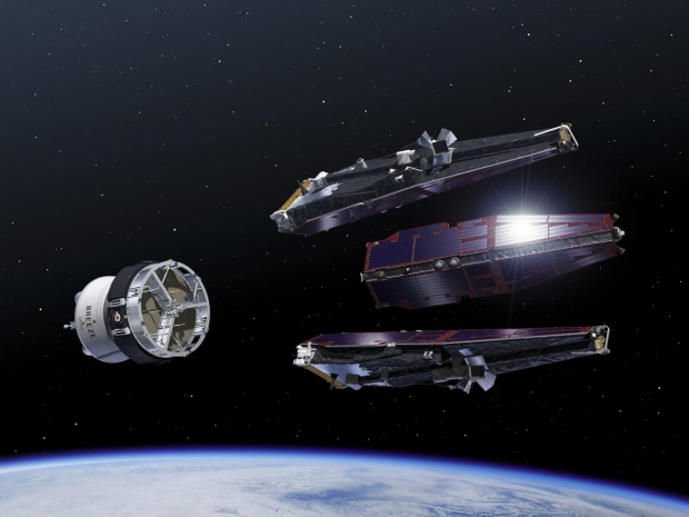
Image: An artist’s concept of ESA’s Swarm mission being deployed. This image was taken from a 2015 workshop on formation flying satellites held at Technische Universiteit Delft in the Netherlands. Extending the swarm paradigm to smallsats and nanosatellites is one step toward future robotic self-assembly. Credit: TU Delft.
Spacecraft operating in swarms optimized for the study of the heliosphere offer tantalizing possibilities in terms of data return. But I think the point that emerges here is flexibility, the notion that coupling a beamed propulsion system to smallsats and nanosats offers a less expensive, modular way to explore targets previously within reach only by expensive flagship missions. I’ll also argue that a large, ground-based laser array is aspirational but not essential to push this paradigm forward.
Issues of self-assembly and sail design are under active study, as is the question of thermal survival for operations close to the Sun. We should continue to explore close solar passes and ‘sundiver’ maneuvers to shorten transit times to targets both relatively near or as far away as the Kuiper Belt. We need test missions to firm up sail materials and operations, even as we experiment with self-assembly of smallsats into larger craft capable of complex operations at target. The result is a modular fleet that can make fast flybys of distant targets or assemble for orbital operations where needed.
The paper is Santi et al., “Swarm of lightsail nanosatellites for Solar System exploration,” available as a preprint.
An Ice Giant’s Possible Oceans
Further fueling my interest in reaching the ice giants is a study in the Journal of Geophysical Research: Planets that investigates the possibility of oceans on the major moons of Uranus. Imaged by Voyager 2, Uranus is otherwise unvisited by our spacecraft, but Miranda, Ariel, Titania, Oberon and Umbriel hold considerable interest given what we are learning about oceans beneath the surface of icy moons. Hence the need to examine the Voyager 2 data in light of updated computer modeling.
Julie Castillo-Rogez (JPL) is lead author of the paper:
“When it comes to small bodies – dwarf planets and moons – planetary scientists previously have found evidence of oceans in several unlikely places, including the dwarf planets Ceres and Pluto, and Saturn’s moon Mimas. So there are mechanisms at play that we don’t fully understand. This paper investigates what those could be and how they are relevant to the many bodies in the solar system that could be rich in water but have limited internal heat.”
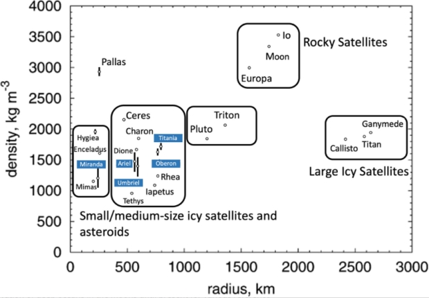
Image: This is Figure 1 from the paper. Caption: Densities and mean radii of the Uranian moons compared to those of other large moons and dwarf planets. Miranda has a low density similar to Saturn’s moon Mimas, whereas the densities of the other Uranian moons are more similar to Saturn’s moons Dione and Rhea. After Hussmann et al. (2006).
The interest is more than theoretical, for as we’ve recently discussed the Planetary Science and Astrobiology Decadal Survey for 2023–2032 has put a Uranus Orbiter and Probe mission on its short list of priorities. A mission to Uranus would open up the prospect for confirming oceans, or the lack of same, within the five large moons. Recent work explored in the Castillo-Rogez paper has made the case that magnetic fields induced by such oceans should be detectable by a Uranus orbiter’s flybys.
Much has happened to call for new modeling of this system. The paper notes recent advances in surface chemistry and geology, revised models of system dynamics, and the knowledge gained on icy bodies in the size range of the Uranian moons as studies have continued on Enceladus and the moons of Saturn as well as Pluto and Charon, not to mention the availability of data from the Dawn mission at Ceres. The team’s modeling produces likely interior structures that are promising for four of the moons.
These moons are indeed small objects, and while Uranus has 27 moons, it is only when we reach the size of Ariel (1160 kilometers) that we can start talking realistically about interior oceans. Titania is the largest of these at 1580 kilometers. The paper argues that of the five largest moons, we can exclude Miranda (470 kilometers) as being too small to sustain the heat to support an internal ocean. But the other four appear promising, revising and contradicting earlier work that had focused primarily on Titania and Oberon in the belief that Ariel, Umbriel, and Miranda would be frozen at present.
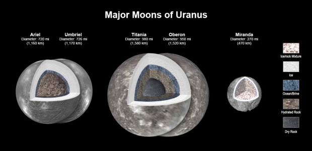
Image: New modeling shows that there likely is an ocean layer in four of Uranus’ major moons: Ariel, Umbriel, Titania, and Oberon. Salty – or briny – oceans lie under the ice and atop layers of water-rich rock and dry rock. Miranda is too small to retain enough heat for an ocean layer. Credit: NASA/JPL-Caltech.
Of the large Uranian moons, Ariel may emerge as the best possibility. From the paper:
Ariel is particularly interesting as a future mission target because of the potential detection of NH3-bearing species on its surface (Cartwright et al., 2021) that could be evidence of recent cryovolcanic activity, considering these species should degrade on a geologically short timescale. Geologic features, visible in Voyager 2 Imaging Science Subsystem images of Ariel, show some evidence for cryovolcanism in the form of double ridges and lobate features that may represent emplaced cryolava (Beddingfield & Cartwright, 2021).
But oceans tens of kilometers deep at Titania and Oberon may yet excite astrobiological interest, depending on what we learn about heat sources here.
Based on current understanding, we conclude that the Uranian moons are more likely to host residual or “relict” oceans than thick oceans. As such, they may be representative of many icy bodies, including Ceres, Callisto, Pluto, and Charon (De Sanctis et al., 2020). The detection and characterization (depth and thickness) of deep oceans inside the Uranian moons… and refined constraint on surface ages would help assess whether these bodies still hold residual heat from a recent resonance crossing event and/or are undergoing tidal heating due to dynamical circumstances that are currently unknown (as was the case at Enceladus before the Cassini mission).
The Uranus Orbiter and Probe mission holds great allure for answering some of these questions. The issue of detection by a spacecraft is still charged, however. The authors note from the outset that an ocean maintained primarily by ammonia would be well below the water freezing point, in which case its electrical conductivity might be too low to register on the UOP’s sensors. In other words, ammonia essentially acts as an antifreeze, with electrical conductivity near zero. Temperatures below ~245 K would mean an ocean would have to be detected by the exposure of deep ocean material, in which case we come back to Ariel as the most likely target for the closest scrutiny.
The paper is Castillo-Rogez et al., “Compositions and Interior Structures of the Large Moons of Uranus and Implications for Future Spacecraft Observations,” JGR Planets Vol. 128, Issue 1 (January 2023). Abstract.
GJ 486b: An Atmosphere around a Rocky M-dwarf Planet?
I might have mentioned the issues involving the James Webb Space Telescope’s MIRI instrument in my earlier post on in-flight maintenance and repair. MIRI is the Mid-Infrared Instrument that last summer had issues with friction in one of the wheels that selects between short, medium and longer wavelengths. Now there seems to be a problem, however slight, that affects the amount of light registered by MIRI’s sensors.
The problems seem minor and are under investigation, which is a good thing because we need MIRI’s capabilities to study systems like GJ 486, where a transiting rocky exoplanet may or may not be showing traces of water in an atmosphere that may or may not be there. MIRI should help sort out the issue, which was raised through observations with another JWST instrument, the Near-Infrared Spectrograph (NIRSpec). The latter shows tantalizing evidence of water vapor, but the problem is untangling whether that signal is coming from the rocky planet or the star.
This points to an important question. GJ 486b is about 30 percent larger than Earth and three times as massive, a rocky super-Earth orbiting its red dwarf host in about 1.5 Earth days. The proximity to the star almost demands tidal lock, with one side forever dark, the other facing the star. If the water vapor NIRSpec is pointing to actually comes from a planetary atmosphere, then that atmosphere copes with surface temperatures in the range of 430 Celsius and the continual bombardment of ultraviolet and X-ray radiation associated with such stars. That would be encouraging news for other systems in which rocky worlds orbit further out, in an M-dwarf’s habitable zone.
Sarah Moran (University of Arizona, Tucson) is lead author of the study, which has been accepted for publication at The Astrophysical Journal Letters:
“We see a signal, and it’s almost certainly due to water. But we can’t tell yet if that water is part of the planet’s atmosphere, meaning the planet has an atmosphere, or if we’re just seeing a water signature coming from the star.”

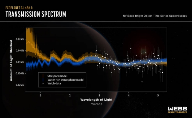
Image: This graphic shows the transmission spectrum obtained by Webb observations of rocky exoplanet GJ 486b. The science team’s analysis shows hints of water vapor; however, computer models show that the signal could be from a water-rich planetary atmosphere (indicated by the blue line) or from starspots from the red dwarf host star (indicated by the yellow line). The two models diverge noticeably at shorter infrared wavelengths, indicating that additional observations with other Webb instruments will be needed to constrain the source of the water signal. Credit: NASA, ESA, CSA, Joseph Olmsted (STScI).
The trick here is that we see GJ 486b transiting its star, allowing astronomers to deploy transmission spectroscopy, in which the light of the star passes through a planet’s atmosphere and affords information about which molecules are found there. This is done only after the star’s spectrum without the transiting planet has been observed. Dips in that spectrum during the transits tell the tale, but in this case we can’t be sure of their source. The flat spectrum during transits rises at short infrared wavelengths and water vapor seems to be the culprit, but stars can have water vapor of their own.
Thus starspots can’t be ruled out, even though there is as yet no evidence that the planet crossed any of these during the two transits for which these data were taken. Even a much hotter G-class star like our Sun can show traces of water vapor in sunspots, which are much cooler than the surrounding surface. An M-dwarf like GJ 486 is far cooler than the Sun, making water vapor detections in its starspots possible.
So imagine the scenario. If we do have an atmosphere here, we have to explain how it can exist despite the continual erosion forced by the star’s heat and irradiation. That would lead one to suspect volcanic replenishment as materials are ejected from the planet’s interior. An already scheduled JWST observational program using MIRI will study the planet’s dayside for signs of an atmosphere that can circulate heat. Hence the significance of fine-tuning MIRI’s small glitches to resolve a big question.
In the case that the upcoming MIRI observations cannot definitely detect an atmosphere, high precision shorter wavelength observations could provide evidence for or against an atmosphere on GJ 486b. Ultimately, our JWST NIRSpec/G395H stellar and transmission spectra, combined with retrievals and stellar models, suggest either an airless planet with a spotted host star or a significant planetary atmosphere containing water vapor. Given the agreement between our stellar modeling and atmospheric retrievals for the spot scenario, this interpretation may have a slight edge over a water-rich atmosphere. However, a true determination of the nature of GJ 486b remains on the horizon, with wider wavelength observations holding the key to this world’s location along the cosmic shoreline.
The paper is Moran et al., “High Tide or Riptide on the Cosmic Shoreline? A Water-Rich Atmosphere or Stellar Contamination for the Warm Super-Earth GJ~486b from JWST Observations,” accepted at The Astrophysical Journal Letters and available as a preprint.

GJ 486b: An Atmosphere around a Rocky M-dwarf Planet?
I might have mentioned the issues involving the James Webb Space Telescope’s MIRI instrument in my earlier post on in-flight maintenance and repair. MIRI is the Mid-Infrared Instrument that last summer had issues with friction in one of the wheels that selects between short, medium and longer wavelengths. Now there seems to be a problem, however slight, that affects the amount of light registered by MIRI’s sensors.
The problems seem minor and are under investigation, which is a good thing because we need MIRI’s capabilities to study systems like GJ 486, where a transiting rocky exoplanet may or may not be showing traces of water in an atmosphere that may or may not be there. MIRI should help sort out the issue, which was raised through observations with another JWST instrument, the Near-Infrared Spectrograph (NIRSpec). The latter shows tantalizing evidence of water vapor, but the problem is untangling whether that signal is coming from the rocky planet or the star.
This points to an important question. GJ 486b is about 30 percent larger than Earth and three times as massive, a rocky super-Earth orbiting its red dwarf host in about 1.5 Earth days. The proximity to the star almost demands tidal lock, with one side forever dark, the other facing the star. If the water vapor NIRSpec is pointing to actually comes from a planetary atmosphere, then that atmosphere copes with surface temperatures in the range of 430 Celsius and the continual bombardment of ultraviolet and X-ray radiation associated with such stars. That would be encouraging news for other systems in which rocky worlds orbit further out, in an M-dwarf’s habitable zone.
Sarah Moran (University of Arizona, Tucson) is lead author of the study, which has been accepted for publication at The Astrophysical Journal Letters:
“We see a signal, and it’s almost certainly due to water. But we can’t tell yet if that water is part of the planet’s atmosphere, meaning the planet has an atmosphere, or if we’re just seeing a water signature coming from the star.”

Image: This graphic shows the transmission spectrum obtained by Webb observations of rocky exoplanet GJ 486b. The science team’s analysis shows hints of water vapor; however, computer models show that the signal could be from a water-rich planetary atmosphere (indicated by the blue line) or from starspots from the red dwarf host star (indicated by the yellow line). The two models diverge noticeably at shorter infrared wavelengths, indicating that additional observations with other Webb instruments will be needed to constrain the source of the water signal. Credit: NASA, ESA, CSA, Joseph Olmsted (STScI).
The trick here is that we see GJ 486b transiting its star, allowing astronomers to deploy transmission spectroscopy, in which the light of the star passes through a planet’s atmosphere and affords information about which molecules are found there. This is done only after the star’s spectrum without the transiting planet has been observed. Dips in that spectrum during the transits tell the tale, but in this case we can’t be sure of their source. The flat spectrum during transits rises at short infrared wavelengths and water vapor seems to be the culprit, but stars can have water vapor of their own.
Thus starspots can’t be ruled out, even though there is as yet no evidence that the planet crossed any of these during the two transits for which these data were taken. Even a much hotter G-class star like our Sun can show traces of water vapor in sunspots, which are much cooler than the surrounding surface. An M-dwarf like GJ 486 is far cooler than the Sun, making water vapor detections in its starspots possible.
So imagine the scenario. If we do have an atmosphere here, we have to explain how it can exist despite the continual erosion forced by the star’s heat and irradiation. That would lead one to suspect volcanic replenishment as materials are ejected from the planet’s interior. An already scheduled JWST observational program using MIRI will study the planet’s dayside for signs of an atmosphere that can circulate heat. Hence the significance of fine-tuning MIRI’s small glitches to resolve a big question.
In the case that the upcoming MIRI observations cannot definitely detect an atmosphere, high precision shorter wavelength observations could provide evidence for or against an atmosphere on GJ 486b. Ultimately, our JWST NIRSpec/G395H stellar and transmission spectra, combined with retrievals and stellar models, suggest either an airless planet with a spotted host star or a significant planetary atmosphere containing water vapor. Given the agreement between our stellar modeling and atmospheric retrievals for the spot scenario, this interpretation may have a slight edge over a water-rich atmosphere. However, a true determination of the nature of GJ 486b remains on the horizon, with wider wavelength observations holding the key to this world’s location along the cosmic shoreline.
The paper is Moran et al., “High Tide or Riptide on the Cosmic Shoreline? A Water-Rich Atmosphere or Stellar Contamination for the Warm Super-Earth GJ~486b from JWST Observations,” accepted at The Astrophysical Journal Letters and available as a preprint.

Voyager as Technosignature
Here’s an image that brings out the philosopher in me, or maybe the poet. It’s Voyager 1, as detected by a new processing system called COSMIC, now deployed at the Very Large Array west of Socorro, New Mexico. Conceived as a way of collecting data in the search for technosignatures, COSMIC (Commensal Open-Source Multimode Interferometer Cluster) taps data from the ongoing VLASS (Very Large Array Sky Survey) project and shunts them into a receiver designed to spot narrow channels, on the order of one hertz wide, to spot possible components of a technosignature.
Technosignatures fire the imagination as we contemplate advanced civilizations going about their business and the possibility of eavesdropping upon them. But for me, the image below conjures up thoughts of human persistence and a gutsy engagement with the biggest issues we face. Why are we here, and where exactly are we in the galaxy? In the cosmos? Spacecraft like the Voyagers were part of the effort to explore the Solar System, but they now push into realms not intended by their designers. And here we have the detection of doughty Voyager 1, still working the mission, somehow still sending us priceless information.
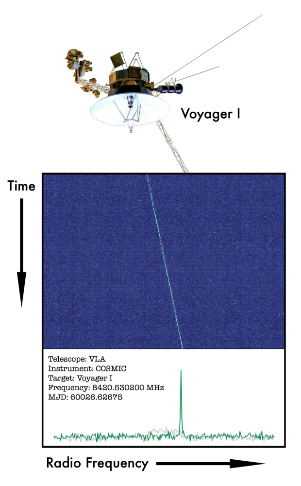
Image: The detection of the Voyager I spacecraft using the COSMIC instrument on the VLA. Launched in 1977, the Voyager I spacecraft is now the most distant piece of human technology ever sent into space, currently around 14.8 billion miles from Earth. Voyager’s faint radio transmitter is difficult to detect even with the largest telescopes, and represents an ideal human “technosignature” for testing the performance of SETI instruments. The detection of Voyager’s downlink gives the COSMIC team high confidence that the system can detect similar artificial transmitters potentially arising from distant extraterrestrial civilizations. Credit: SETI Institute.
Voyager 1 is thus a dry run for a technosignature detection, and COSMIC is said to offer a sensitivity a thousand times more comprehensive than any previous SETI search. The detection is unmistakable, combining and verifying the operation of the individual antennas that comprise the array to show the carrier signal and sideband transmissions from the spacecraft. The most distant of all human-made objects, Voyager 1 is now 24 billion kilometers from home. For one participant in COSMIC, the spacecraft demonstrates what can be done by combing through the incoming datastream of VLASS. Thus Jack Hickish (Real Time Radio Systems Ltd):
“The detection of Voyager 1 is an exciting demonstration of the capabilities of the COSMIC system. It is the culmination of an enormous amount of work from an international team of scientists and engineers. The COSMIC system is a fantastic example of using modern general-purpose compute hardware to augment the capabilities of an existing telescope and serves as a testbed for technosignatures research on upcoming radio telescopes such as NRAO’s Next Generation VLA.”
COSMIC is the result of collaboration between The SETI Institute (working with the National Radio Astronomy Observatory) and the Breakthrough Listen Initiative. The key here is efficiency – the technosignature search draws on data already being taken for other reasons, and given the challenge of obtaining large amounts of telescope time, an offshoot method of tracking pulsed and transient signals simply makes use of existing resources, with approximately ten million star systems within its scope.
Technosignatures are fascinating, but I come back to Voyager. We’ve gotten used to the scope of its achievement, but what fires the imagination is the details. It wasn’t all that long ago, for example, that controllers decided to switch to the use of the spacecrafts’ backup thrusters. The reason: The primary thrusters, having gone through almost 350,000 thruster cycles, were pushing their limits. When the backup thrusters were fired in 2017, the spacecraft had been on their way for forty years. The “trajectory correction maneuver,” or TCM, thrusters built by Aerojet Rocketdyne (also used on Cassini, among others), dormant since Voyager 1’s swing by Saturn in 1980, worked flawlessly.
In his book The Interstellar Age (Dutton, 2015), Jim Bell came up with an interesting future possibility for the Voyagers before we lose them forever. Bell worked as an intern on the Voyager science support team at JPL starting in 1980, and he would like to see some of the results of the mission stored up for a potentially wider audience. Right now there is nothing aboard each spacecraft that tells their stories. Bell quotes Jon Lomberg, who worked on the Voyager Golden Records and has advanced the idea of a digital message to be uploaded to New Horizons:
‘One thing I wish could have been on the Voyager record… is that I wish we could have had something of ‘here’s what Voyager was and here’s what Voyager found,’ because it’s one of the best things human beings have ever done. If they ever find Voyager they won’t know about its mission. They won’t know what it did, and that’s sad.’
And Bell goes on to say:
…let’s try to upload the Earth-Moon portrait; the historic first close-up photos of Io’s volcanoes and Europa and Ganymede’s cracked icy shells; the smoggy haze of Titan; the enormous cliffs of Miranda; the strange cantaloupe and geyser terrain of Triton; the swirling storms of Jupiter, Saturn and Neptune; the elegant, intricate ring systems of all four giant planets; the family portrait of our solar system. Let’s arm our Voyagers with electronic postcards so they can properly tell their tales, should any intelligence ever find them.
Could images be uploaded to the Voyager tape recorders at some point before communication is lost? It’s an intriguing thought about a symbolic act, but whether possible or not, it reminds us of the distances the Voyagers have thus far traveled and the presence of something built here on Earth that will keep going, blind and battered but more or less intact, for eons.