Centauri Dreams
Imagining and Planning Interstellar Exploration
A Radium Age Take on the ‘Wait Equation’
If you’ll check Project Gutenberg, you’ll find Bernhard Kellermann’s novel The Tunnel. Published in 1913 by the German house S. Fischer Verlag and available on Gutenberg only in its native tongue (finding it in English is a bit more problematic, although I’ve seen it on offer from online booksellers occasionally), the novel comes from an era when the ‘scientific romance’ was yielding to an engineering-fueled uneasiness with what technology was doing to social norms.

Kellermann was a poet and novelist whose improbable literary hit in 1913, one of several in his career, was a science fiction tale about a tunnel so long and deep that it linked the United States with Europe. It was written at a time when his name was well established among readers throughout central Europe. His 1908 novel Ingeborg saw 131 printings in its first thirty years, so this was a man often discussed in the coffee houses of Berlin and Vienna.
Image: Author Bernhard Kellermann, author of The Tunnel and other popular novels as well as poetry and journalistic essays. Credit: Deutsche Fotothek of the Saxon State Library / State and University Library Dresden (SLUB).
The Tunnel sold 10,000 copies in its first four weeks, and by six months later had hit 100,000, becoming the biggest bestseller in Germany in 1913. It would eventually appear in 25 languages and sell over a million copies. By way of comparison – and a note about the vagaries of fame and fortune – Thoman Mann’s Death in Venice, also published that year, sold 18,000 copies for the whole year, and needed until the 1930s to reach the 100,000 mark. Short-term advantage: Kellermann.
I mention this now obscure novel for a couple of reasons. For one thing, it’s science fiction in an era before popular magazines filled with the stuff had begun to emerge to fuel the public imagination. This is the so-called ‘radium age,’ recently designated as such by Joshua Glenn, whose series for MIT press reprints works from the period.
We might define an earlier era of science fiction, one beginning with the work of, say, Mary Wollstonecraft Shelley and on through H. G. Wells, and a later one maybe dating from Hugo Gernsback’s creation of Amazing Stories in 1926 (Glenn prefers to start the later period at 1934, which is a few years before the beginning of the Campbell era at Astounding, where Heinlein, Asimov and others would find a home), but in between is the radium age. Here’s Glenn, from a 2012 article in Nature:
[Radium age novels] depict a human condition subverted or perverted by science and technology, not improved or redeemed. Aldous Huxley’s 1932 Brave New World, with its devastating satire on corporate tyranny, behavioral conditioning and the advancement of biotechnology, is far from unique. Radium-age sci-fi tends towards the prophetic and uncanny, reflecting an era that saw the rise of nuclear physics and the revelation that the familiar — matter itself — is strange, even alien. The 1896 discovery of radioactivity, which led to the early twentieth-century insight that the atom is, at least in part, a state of energy, constantly in movement, is the perfect metaphor for an era in which life itself seemed out of control.
All of which is interesting to those of us of a historical bent, but The Tunnel struck me forcibly because of the year in which it was published. Radiotelegraphy, as it was then called, had just been deployed across the Atlantic on the run from New York to Germany, a distance (reported in Telefunken Zeitschrift in April of that year) of about 6,500 kilometers. Communicating across oceans was beginning to happen, and it is in this milieu that The Tunnel emerged to give us a century-old take on what we in the interstellar flight field often call the ‘wait equation.’
How long do we wait to launch a mission given that new technology may become available in the future? Kellermann’s plot involved the construction of the tunnel, a tale peppered with social criticism and what German author Florian Illies calls ‘wearily apocalyptic fantasy.’ Illies is, in fact, where I encountered Kellermann, for his 2013 title 1913: The Year Before the Storm, now available in a deft new translation, delves among many other things into the literary and artistic scene of that fraught year before the guns of August. This is a time of Marcel Duchamp, of Picasso, of Robert Musil. The Illies book is a spritely read that I can’t recommend too highly if you like this sort of thing (I do).
In The Tunnel, it takes Kellermann’s crews 24 years of agonizing labor, but eventually the twin teams boring through the seafloor manage to link up under the Atlantic, and two years later the first train makes the journey. It’s a 24 hour trip instead of the week-long crossing of the average ocean liner, a miracle of technology. But it soon becomes apparent that nobody wants to take it. For even as work on the tunnel has proceeded, aircraft have accelerated their development and people now fly between New York and Berlin in less than a day.
The ‘wait equation’ is hardly new, and Kellermann uses it to bring all his skepticism about technological change to the fore. Here’s how Florian Illies describes the novel:
…Kellermann succeeds in creating a great novel – he understands the passion for progress that characterizes the era he lives in, the faith in the technically feasible, and at the same time, with delicate irony and a sense for what is really possible, he has it all come to nothing. An immense utopian project that is actually realized – but then becomes nothing but a source of ridicule for the public, who end up ordering their tomato juice from the stewardess many thousand meters not under but over the Atlantic. According to Kellermann’s wise message, we would be wise not to put our utopian dreams to the test.
Here I’ll take issue with Illies, and I suppose Kellermann himself. Is the real message that utopian dreams come to nothing? If so, then a great many worthwhile projects from our past and our future are abandoned in service of a judgment call based on human attitudes toward time and generational change. I wonder how we go about making that ‘wait equation’ decision. Not long ago, Jeff Greason told Bruce Dorminey that it would be easier to produce a mission to the nearest star that took 20 years than to figure out how to fund, much less to build, a mission that would take 200 years.
He’s got a point. Those of us who advocate long-term approaches to deep space also have an obligation to reckon with the hard practicalities of mission support over time, which is not only a technical but a sociological issue that makes us ask who will see the mission home. But I think we can also see philosophical purpose in a different class of missions that our species may one day choose to deploy. Missions like these:
1) Advanced AI will at some point negate the question of how long to wait if we assume spacecraft that can seamlessly acquire knowledge and return it to a network of growing information, a nascent Encyclopedia Galactica of our own devising that is not reliant on Earth. Ever moving outward, it would produce a wavefront of knowledge that theoretically would be useful not just to ourselves but whatever species come after us.
2) Human missions intended as generational, with no prospect of return to the home world, also operate without lingering connections to controllers left behind. Their purpose may be colonization of exoplanets, or perhaps simple exploration, with no intention of returning to planetary surfaces at all. Indeed, some may choose to exploit resources, as in the Oort Cloud, far from inner systems, separating from Earth in the service of particular research themes or ideologies.
3) Missions designed to spread life have no necessary connection with Earth once launched. If life is rare in the galaxy, it may be within our power to spread simple organisms or even revive/assemble complex beings, a melding of human and robotics. An AI crewed ship that raises human embryos on a distant world would be an example, or a far simpler fleet of craft carrying a cargo of microorganisms. Such journeys might take millennia to reach their varied targets and still achieve their purpose. I make no statement here about the wisdom of doing this, only noting it as a possibility.
In such cases, creating a ‘wait equation’ to figure out when to launch loses force, for the times involved do not matter. We are not waiting for data in our lifetimes but are acting through an imperative that operates on geological timeframes. That is to say, we are creating conditions that will outlast us and perhaps our civilizations, that will operate over stellar eras to realize an ambition that transcends humankind. I’m just brainstorming here, and readers may want to wrangle over other mission types that fit this description.
But we can’t yet launch missions like these, and until we can, I would want any mission to have the strongest possible support, financial and political, here on the home world if we are talking about many decades for data return. It’s hard to forget the scene in Robert Forward’s Rocheworld where at least one political faction actively debates turning off the laser array that the crew of a starship approaching Barnard’s Star will use to brake into the planetary system there. Political or social change on the home world has to be reckoned into the equation when we are discussing projects that demand human participation from future generations.
These things can’t be guaranteed, but they can be projected to the best of our ability, and concepts chosen that will maintain scientific and public interest for the duration needed. You can see why mission design is also partly a selling job to the relevant entities as well as to the public, something the team working on a probe beyond the heliopause at the Johns Hopkins University Applied Physics Lab knows all too well.
Back to Bernhard Kellermann, who would soon begin to run afoul of the Nazis (his novel The Ninth November was publicly burned in Germany). He would later be locked out of the West German book trade because of his close ties with the East German government and his pro-Soviet views. He died in Potsdam in 1951.

Image: A movie poster showing Richard Dix and C. Aubrey Smith discussing plans for the gigantic project in Transatlantic Tunnel (1935). Credit: IMDB.
The Tunnel became a curiosity, and spawned an even more curious British movie by the same name (although sometimes found with the title Transatlantic Tunnel) starring Richard Dix and Leslie Banks. In the 1935 film, which is readily available on YouTube or various streaming platforms, the emphasis is on a turgid romance, pulp-style dangers overcome and international cooperation, with little reflection, if any, on the value of technology and how it can be superseded.
The interstellar ‘wait equation’ could use a movie of its own. I for one would like to see a director do something with van Vogt’s “Far Centaurus,” the epitome of the idea.
The Glenn paper is “Science Fiction: The Radium Age,” Nature 489 (2012), 204-205 (full text).

Microlensing: Expect Thousands of Exoplanet Detections
We just looked at how gravitational microlensing can be used to analyze the mass of a star, giving us a method beyond the mass-luminosity relationship to make the call. And we’re going to be hearing a lot more about microlensing, especially in exoplanet research, as we move into the era of the Nancy Grace Roman Space Telescope (formerly WFIRST), which is scheduled to launch in 2027. A major goal for the instrument is the expected discovery of exoplanets by the thousands using microlensing. That’s quite a jump – I believe the current number is less than 100.
For while radial velocity and transit methods have served us well in establishing a catalog of exoplanets that now tops 5000, gravitational microlensing has advantages over both. When a stellar system occludes a background star, the lensing of the latter’s light can tell us much about the planets that orbit the foreground object. Whereas radial velocity and transits work best when a planet is in an orbit close to its star, microlensing can detect planets in orbits equivalent to the gas giants in our system.
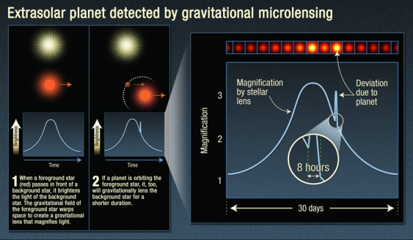
Image: This infographic explains the light curve astronomers detect when viewing a microlensing event, and the signature of an exoplanet: an additional uptick in brightness when the exoplanet lenses the background star. Credit: NASA / ESA / K. Sahu / STScI).
Moreover, we can use the technique to detect lower-mass planets in such orbits, planets far enough, for example, from a G-class star to be in its habitable zone, and small enough that the radial velocity signature would be tricky to tease out of the data. Not to mention the fact that microlensing opens up vast new areas for searching. Consider: TESS deliberately works with targets nearby, in the range of 100 light years. Kepler’s stars averaged about 1000 light years. Microlensing as planned for the Roman instrument will track stars, 200 million of them, at distances around 10,000 light years away as it looks toward the center of the Milky Way.
So this is a method that lets us see planets at a wide range of orbital distances and in a wide range of sizes. The trick is to work out the mass of both star and planet when doing a microlensing observation, which brings machine learning into the mix. Artificial intelligence algorithms can parse these data to speed the analysis, a major plus when we consider how many events the Roman instrument is likely to detect in its work.
The key is to find the right algorithms, for the analysis is by no means straightforward. Microlensing signals involve the brightening of the light from the background star over time. We can call this a ‘light curve,’ which it is, making sure to distinguish what’s going on here from the transit light curve dips that help identify exoplanets with that method. With microlensing, we are seeing light bent by the gravity of the foreground star, so that we observe brightening, but also splitting of the light, perhaps into various point sources, or even distorting its shape into what is called an Einstein ring, named of course after the work the great physicist did in 1936 in identifying the phenomenon. More broadly, microlensing is implied by all his work on the curvature of spacetime.
However the light presents itself, untangling what is actually present at the foreground object is complicated because more than one planetary orbit can explain the result. Astronomers refer to such solutions as degeneracies, a term I most often see used in quantum mechanics, where it refers to the fact that multiple quantum states can emerge with the same energy, as happens, for example, when an electron orbits one or the other way around a nucleus. How to untangle what is happening?
A new paper in Nature Astronomy moves the ball forward. It describes an AI algorithm developed by graduate student Keming Zhang at UC-Berkeley, one that presents what the researchers involved consider a broader theory that incorporates how such degeneracies emerge. Here is the university’s Joshua Bloom, in a blog post from last December, when the paper was first posted to the arXiv site:
“A machine learning inference algorithm we previously developed led us to discover something new and fundamental about the equations that govern the general relativistic effect of light- bending by two massive bodies… Furthermore, we found that the new degeneracy better explains some of the subtle yet pervasive inconsistencies seen [in] real events from the past. This discovery was hiding in plain sight. We suggest that our method can be used to study other degeneracies in systems where inverse-problem inference is intractable computationally.”
What an intriguing result. The AI work grows out of a two-year effort to analyze microlensing data more swiftly, allowing the fast determination of the mass of planet and star in a microlensing event, as well as the separation between the two. We’re dealing with not one but two brightness peaks in the brightness of the background star, and trying to deduce from this an orbital configuration that produced the signal. Thus far, the different solutions produced by such degeneracies have been ambiguous.
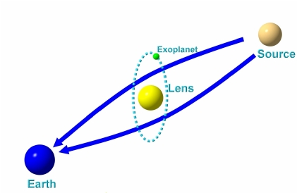
Image: Seen from Earth (left), a planetary system moving in front of a background star (source, right) distorts the light from that star, making it brighten as much as 10 or 100 times. Because both the star and exoplanet in the system bend the light from the background star, the masses and orbital parameters of the system can be ambiguous. An AI algorithm developed by UC Berkeley astronomers got around that problem, but it also pointed out errors in how astronomers have been interpreting the mathematics of gravitational microlensing. Credit: Research Gate.
Zhang and his fellow researchers applied microlensing data from a wide variety of orbital configurations to run the new AI algorithm through its paces. Let’s hear from Zhang himself:
“The two previous theories of degeneracy deal with cases where the background star appears to pass close to the foreground star or the foreground planet. The AI algorithm showed us hundreds of examples from not only these two cases, but also situations where the star doesn’t pass close to either the star or planet and cannot be explained by either previous theory. That was key to us proposing the new unifying theory.”
Thus to existing known degeneracies labeled ‘close-wide’ and ‘inner-outer,’ Zhang’s work adds the discovery of what the team calls an ‘offset’ degeneracy. An underlying order emerges, as the paper notes, from the offset degeneracy. In the passage from the paper below, a ‘caustic’ defines the boundary of the curved light signal. Italics mine:
…the offset degeneracy concerns a magnification-matching behaviour on the lens-axis and is formulated independent of caustics. This offset degeneracy unifies the close-wide and inner-outer degeneracies, generalises to resonant topologies, and upon re- analysis, not only appears ubiquitous in previously published planetary events with 2-fold degenerate solutions, but also resolves prior inconsistencies. Our analysis demonstrates that degenerate caustics do not strictly result in degenerate magnifications and that the commonly invoked close-wide degeneracy essentially never arises in actual events. Moreover, it is shown that parameters in offset degenerate configurations are related by a simple expression. This suggests the existence of a deeper symmetry in the equations governing 2-body lenses than previously recognised.
The math in this paper is well beyond my pay grade, but what’s important to note about the passage above is the emergence of a broad pattern that will be used to speed the analysis of microlensing lightcurves for future space-and ground-based observations. The algorithm provides a fit to the data from previous papers better than prior methods of untangling the degeneracies, but it took the power of machine learning to work this out.
It’s also noteworthy that this work delves deeply into the mathematics of general relativity to explore microlensing situations where stellar systems include more than one exoplanet, which could involve many of them. And it turns out that observations from both Earth and the Roman telescope – two vantage points – will make the determination of orbits and masses a good deal more accurate. We can expect great things from Roman.
The paper is Zhang et al., “A ubiquitous unifying degeneracy in two-body microlensing systems,” Nature Astronomy 23 May 2022 (abstract / preprint).
Proxima Centauri: Microlensing Yields New Data
It’s not easy teasing out information about a tiny red dwarf star, even when it’s the closest star to the Sun. Robert Thorburn Ayton Innes (1861-1933), a Scottish astronomer, found Proxima using a blink comparator in 1915, noting a proper motion similar to Alpha Centauri (4.87” per year), with Proxima about two degrees away from the binary. Finding out whether the new star was actually closer than Centauri A and B involved a competition with a man with a similarly august name, Joan George Erardus Gijsbertus Voûte, a Dutch astronomer working in South Africa. Voûte’s parallax figures were more accurate, but Innes didn’t wait for debate, and proclaimed the star’s proximity, naming it Proxima Centaurus.
The back and forth over parallax and the subsequent careers of both Innes and Voûte make for interesting reading. I wrote both astronomers up back in 2013 in Finding Proxima Centauri, but I’ll send you to my source for that article, Ian Glass (South African Astronomical Observatory), who published the details in the magazine African Skies (Vol. 11 (2007), p. 39). You can find the abstract here.
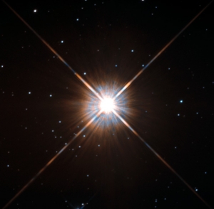
Image: Shining brightly in this Hubble image is our closest stellar neighbour: Proxima Centauri. Although it looks bright through the eye of Hubble, as you might expect from the nearest star to the Solar System, the star is not visible to the naked eye. Its average luminosity is very low, and it is quite small compared to other stars, at only about an eighth of the mass of the Sun. However, on occasion, its brightness increases. Proxima is what is known as a “flare star”, meaning that convection processes within the star’s body make it prone to random and dramatic changes in brightness. The convection processes not only trigger brilliant bursts of starlight but, combined with other factors, mean that Proxima Centauri is in for a very long life. Astronomers predict that this star will remain on the main sequence for another four trillion years, some 300 times the age of the current Universe. These observations were taken using Hubble’s Wide Field and Planetary Camera 2 (WFPC2). Credit: NASA/ESA.
It’s a long way from blink comparators to radial velocity measurements, the latter of which enabled our first exoplanet discoveries back in the 1990s, measuring how the gravitational pull of an orbiting planet could pull its parent star away from us, then towards us on the other side of the orbit, with all the uncertainties that implies. We’re still drilling into the details of Proxima Centauri, and radial velocity occupies us again today. The method depends on the mass of the star, for if we know that, we can then make inferences about the mass of the planets we find around it.
Thus the discovery of Proxima Centauri’s habitable zone planet, Proxima b, a planet we’d like to know much more about given its enticing minimum mass of about 1.3 Earths and an orbital period of just over 11 days. Radial velocity methods at exquisite levels of precision rooted out Proxima b and continue to yield new discoveries.
We’re learning a lot about Alpha Centauri itself – the triple system of Proxima and the central binary Centauri A and B. Just a few years ago, Pierre Kervella and team were able to demonstrate what had previously been only a conjecture, that Proxima Centauri was indeed gravitationally bound to Centauri A and B. The work was done using high-precision radial velocity measurements from the HARPS spectrograph. But we still had uncertainty about the precise value of Proxima’s mass, which had in the past been extrapolated from its luminosity.
This mass-luminosity relation is useful when we have nowhere else to turn, but as a paper from Alice Zurlo (Universidad Diego Portales, Chile) explains, there are significant uncertainties in these values, which point to higher error bars the smaller the star in question. As we learn more about not just other planets but warm dust belts around Proxima Centauri, we need a better read on the star’s mass, and this leads to the intriguing use to which Zurlo and team have put gravitational microlensing.
Here we’re in new terrain. The gravitational deflection of starlight is well demonstrated, but to use it, we need to have a background object move close enough to Proxima Centauri so that the latter can deflect its light. A measurement of this kind was recently made on the star Stein 3051 B, a white dwarf, using data from the Hubble instrument, the first use of gravitational lensing to measure the mass of a star beyond our Solar System. Zurlo and team have taken advantage of microlensing events at Proxima involving two background stars, one in 2014 (source 1), the other two years later (source 2), but the primary focus of their work is with the second event.
Using the Spectro-Polarimetric High-contrast Exoplanet REsearch instrument (SPHERE) at the Very Large Telescope at Cerro Paranal in Chile, the researchers observed Proxima Centauri and the background stars from March of 2015 to June of 2017. You can see Proxima in the image below, with the two background stars. In the caption, IRDIS refers to the near-infrared imager and spectrograph which is a part of the SPHERE/VLT installation.
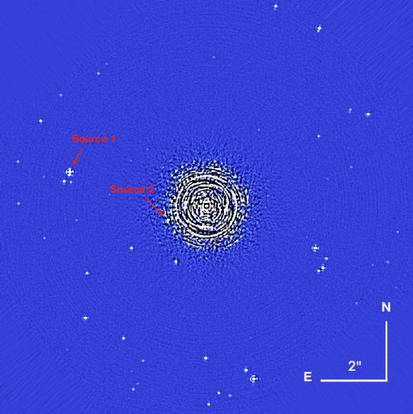
Image: This is Figure 1 from the paper. Caption: IRDIS FoV for the April 2016 epoch. The image is derotated, median combined, and cleaned with a spatial filter. At the center of the image, inside the inner working angle (IWA), the speckle pattern dominates, in the outer part of the image our reduction method prevents the elongation of the stars’ point spread functions (PSFs). The bars in the lower right provide the spatial scale. North is up and East is to the left. Credit: Zurlo et al.
The extraordinary precision of measurement needed here is obvious, and the mechanics of making it happen are described in painstaking detail in the paper. The authors note that the SPHERE observations will not be further refined because the background star they call Source 2 is no longer visible on the instrument’s detector. Nonetheless:
The precision of the astrometric position of this source is the highest ever reached with SPHERE, thanks to the exquisite quality of the data, and the calibration of the detector parameters with the large population of background stars in the FoV. Over the next few years, Proxima Cen will be followed up to provide a better estimation of its movement on the sky. These data will be coupled with observations from HST and Gaia to take advantage of future microlensing events.
The results of the two-year monitoring program show deflection of the background sources’ light consistent with our tightest yet constraints on the mass of Proxima Centauri. The value is 0.150 solar masses, with possible error in the range of +0.062 to -0.051, or roughly 40%. This is, the authors note, “the first and the only currently possible measurement of the gravitational mass of Proxima Centauri.”
The previous value drawn from mass-luminosity figures was 0.12 ± 0.02 M?. What next? While Source 2 may be out of the picture using the SPHERE installation, the authors add that Gaia measurements of the proper motion and parallax of that star may further refine the analysis. Future microlensing will have to wait, for no star as bright as Source 2 will pass within appropriate range of Proxima for another 20 years.
The paper is Zurlo et al., “The gravitational mass of Proxima Centauri measured with SPHERE from a microlensing event,” Monthly Notices of the Royal Astronomical Society Vol. 480, Issue 1 (October, 2018), 236-244 (full text). The paper on Proxima Centauri’s orbit in the Alpha Centauri system is Kervella et al., “Proxima’s orbit around ??Centauri,” Astronomy & Astrophysics Volume 598 (February 2017) L7 (abstract).

“If Loud Aliens Explain Human Earliness, Quiet Aliens Are Also Rare”: A review
What can we say about the possible appearance and spread of civilizations in the Milky Way? There are many ways of approaching the question, but in today’s essay, Dave Moore focuses on a recent paper from Robin Hanson and colleagues, one that has broad implications for SETI. A regular contributor to Centauri Dreams, Dave was born and raised in New Zealand, spent time in Australia, and now runs a small business in Klamath Falls, Oregon. He adds: “As a child, I was fascinated by the exploration of space and science fiction. Arthur C. Clarke, who embodied both, was one of my childhood heroes. But growing up in New Zealand in the ‘60s, such things had little relevance to life, although they did lead me to get a degree in biology and chemistry.” Discovering like-minded people in California, he expanded his interest in SETI and began attending conferences on the subject. In 2011, he published a paper in JBIS, which you can read about in Lost in Time and Lost in Space.
by Dave Moore
I consider the paper “If Loud Aliens Explain Human Earliness, Quiet Aliens Are Also Rare,” by Robin Hanson, Daniel Martin, Calvin McCarter, and Jonathan Paulson, a significant advance in addressing the Fermi Paradox. To explain exactly why, I need to go into its background.
Introduction and History
In our discussions and theories about SETI, the Fermi paradox hangs over them all like a sword of Damocles, ready to fall and cut our assumptions to pieces with the simple question, where are the aliens? There is no reason not to suppose that Earth-like planets could not have formed billions of years before Earth did and that exosolar technological civilizations (ETCs) could not have arisen billions of years ago and spread throughout the galaxy. So why then don’t we see them? And why haven’t they visited us, given the vast expanse of time that has gone by?
Numerous papers and suggestions have tried to address this conundrum, usually ascribing it to some form of alien behavior, or that the principle of mediocrity doesn’t apply, and intelligent life is a very rare fluke.
The weakness of the behavioral arguments is they assume universal alien behaviors, but given the immense differences we expect from aliens—they will be at least as diverse as life on Earth—why would they all have the same motivation? It only takes one ETC with the urge to expand, and diffusion scenarios show that it’s quite plausible for an expansive ETC to spread across the galaxy in a fraction (tens of millions of years) of the time in which planets could have given rise to ETCs (billions of years).
And there is not much evidence that the principle of mediocrity doesn’t apply. Our knowledge of exosolar planets shows that while Earth as a type of planet may be uncommon, it doesn’t look vanishingly rare, and we cannot exclude from the evidence we have that other types of planets cannot give rise to intelligent life.
Also, modest growth rates can produce Kardeshev III levels of energy consumption in the order of tens of thousands of years, which in cosmological terms is a blink of the eye.
In 2010, I wrote a paper for JBIS modeling the temporal dispersion of ETCs. By combining this with other information, in particular diffusion models looking at the spread of civilizations across the galaxy, it was apparent that it was just not possible for spreading ETCs to occur with any frequency at all if they lasted longer than about 20,000 years. Longer than that and at some time in Earth’s history, they would have visited/colonized us by now. So, it looks like we are the first technological civilization in our galaxy. This may be disappointing for SETI, but there are other galaxies out there—at least as many as there are stars in our galaxy.
My paper was a very basic attempt to deduce the distribution of ETCs from the fact we haven’t observed any yet. Robin Hanson et al’s paper, however, is a major advance in this area as it builds a universe-wide quantitative framework to frame this lack of observational evidence and produces some significant conclusions.
It starts with the work done by S. Jay Olsen. In 2015, Olson began to bring out a series of papers assuming the expansion of ETCs and modeling their distributions. He reduced all the parameters of ETC distribution down to two: (?), the rate at which civilizations appeared over time, and (v) their expansion rate, which was assumed to be similar for all civilizations as ultimately all rocketry is governed by the same laws of physics. Olsen varied these two parameters and calculated the results for the following: the ETC-saturated fraction of the universe, the expected number and angular size of their visible domains, the probability that at least one domain is visible, and finally the total expected fraction of the sky eclipsed by expanding ETCs.
In 2018, Hanson et al took Olsen’s approach but incorporated the idea of bringing in the Hard Steps Power Law into modeling the appearance rate of ETCs, which they felt was more accurate and predictive than the rate-over-time models Olsen used.
The Hard Steps Power Law
The Hard Steps power law was first introduced in 1953 to model the appearance of cancer cells. To become cancerous an individual cell must undergo a number of specific mutations (hard steps i.e. improbable steps) in a certain order. The average time for each mutation is longer than a human lifetime, but we have a lot of cells in our body, so 40% of us develop cancer, the result of a series of improbabilities in a given cell.
If you think of all the planets in a galaxy that life can evolve on as cells and the ones that an ETC arises on being cancerous, you get the idea. The Hard Steps model is a power law, so the chances of an outcome happening in a given period of time is the inverse of the chance of a step happening (its hardness) to the power of the number of steps. Therefor the chance of anything happening in a given time goes down very rapidly with the number of hard steps required.
In Earth’s case, the given period of time is about 5.5 billion years, the time from Earth’s origin until the time that a runaway greenhouse sets in about a billion years from now.
The Number of Hard Steps in our Evolution
In 1983 Brandon Carter was looking into how likely it was for intelligent life to arise on Earth, and he thought that due to the limitations on the time available this could be modeled as a hard step problem. To quote:
This means that some of the essential steps (such as the development of eukaryotes) in the evolution process leading to the ultimate emergence of intelligent life would have been hard, in the sense of being against the odds in the available time, so that they are unlikely to have been achieved in most of the earth-like planets that may one day be discovered in nearby extra-solar systems.
Carter estimated that the number of hard steps it took to reach our technological civilization was six: biogenesis, the evolution of bacteria, eukaryotes, combogenisis [sex], metazoans, and intelligence. This, he concluded, seemed the best fit for the amount of time that had taken for us to evolve. There has been much discussion and examination of the number of hard steps in the literature, but the idea has held up fairly well so Hanson et al varied the number of hard steps around six as one of their model variables.
The Paper
The Hanson paper starts out by dividing ETCs into two categories: loud aliens and quiet aliens. To quote:
Loud (or “expansive”) aliens expand fast, last long, and make visible changes to their volumes. Quiet aliens fail to meet at least one of these criteria. As quiet aliens are harder to see, we are forced to accept uncertain estimates of their density, via methods like the Drake equation. Loud aliens, by contrast, are far more noticeable if they exist at any substantial density.
The paper then puts aside the quiet aliens as they are, with our current technology, difficult to find and focuses on the loud ones and, in a manner similar to Olsen, runs models but with the following three variables:
i) The number of hard steps required for an ETC to arise.
ii) The conversion rate of a quiet ETC into a loud, i.e. visible, one.
iii) The expansion speed of a civilization.
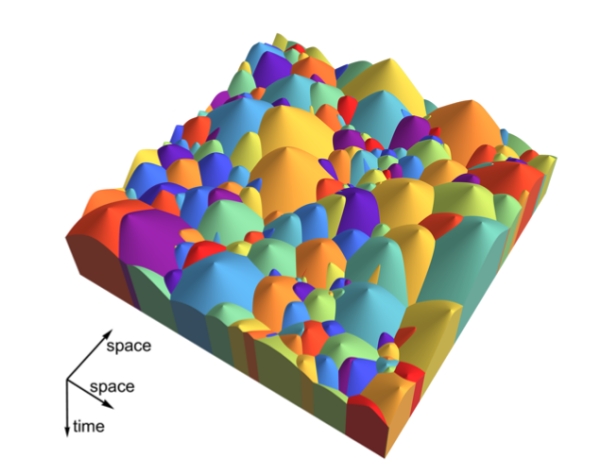
In their models, (like the one illustrated below) a civilization arises. At some point, it converts into an expansive civilization and spreads out until it abuts a neighbor at which point it stops. Further civilizations in the volume that is controlled are prevented from happening. Results showing alien civilizations that are visible from our point of view are discarded, narrowing the range of these variables. (Note: time runs forward going down the page.)
Results
In a typical run with parameters resulting in them not being visible to us, expansive civilizations now control 40-50% of the universe, and they will finish up controlling something like a million galaxies when we meet one of them in 200 million year’s time. (Note, this paradoxical result is due to the speed of light. They control 40-50% of the universe now, but the electromagnetic radiation from their distant galaxies has yet to reach us.)
From these models, three main outcomes become apparent:
Our Early Appearance
The Hard Step model itself contains two main parameters, number of steps and the time in which they must be concluded in. By varying these parameters, Hanson et al showed that, unless one assumes fewer than two hard steps (life and technological civilizations evolve easily) and a very restrictive limit on planet habitability lifetimes, then the only way to account for a lack of visible civilizations is to assume we have appeared very early in the history of civilizations arising in the universe. (In keeping with the metaphor, we’re a childhood cancer.)
All scenarios that show a higher number of hard steps than this greatly favor a later arrival time of ETCs, so an intelligent life form producing a technological civilization is at this stage of the universe is a low probability event.
Chances of other civilizations in our galaxy
Another result coming from their models is that the higher the chance of an expansive civilization evolving from a quiet civilization, the less the chance there is of there being any ETCs aside from us in our galaxy. To summarize their findings: assuming a generous million year average duration for a quiet civilization to become expansive, very low transition chances (p) are needed to estimate that even one other civilization was ever active anywhere along our past light cone (p < 10?3), or existed in our galaxy (p < 10?4), or is now active in our galaxy (p < 10?7).
For SETI to be successful, there needs to be a loud ETC close by, and for one to be close by, the conversion rate of quiet civilizations to expansive, loud ones must be in the order of one per billion. This is not a good result pointing to SETI searches being productive.
Speed of expansion
The other variable used in the models is the speed of expansion. Under most assumptions, expansive civilizations cover significant portions of the sky. However, when taking into account the speed of light, the further distant these civilizations are, the earlier they must form for us to see them. One of the results of this relativistic model is that the slower civilizations expand on average, the more likely we are to see them.
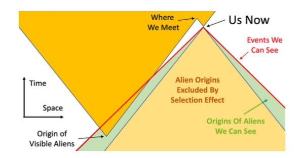
This can be demonstrated with the above diagram. The orange portion of the diagram shows the origin and expansion of an ETC at a significant proportion of the speed of light. We—by looking out into space are also looking back in time—can only see what is in our light cone (that which is below the red line), so we see the origin of our aliens (say one billion years ago) and their initial spread up to about half that age. After which, the emissions from their spreading civilization have not yet had time to reach us.
The tan triangle represents the area in space from which an ETC spreading at the same rate as the orange aliens would already have arrived at our planet (in which case we would either not exist or we would know about it), so we can assume that there were no expansive aliens having originated in this portion of time and space.
If we make the spread rate a smaller proportion of the speed of light, then this has the effect of making both the orange and tan triangles narrower along the space axis. The size of the tan exclusion area becomes smaller, and the green area, which is the area that can contain observable alien civilizations that haven’t reached us yet, becomes bigger.
You’ll also notice that the narrower orange triangle of the expansive ETC crosses out of out of our light cone at an earlier age, so we’d only see evidence of their civilization from an earlier time.
The authors note that the models rely on us being able to detect the boundaries between expansive civilizations and unoccupied space. If the civilizations are out there, but are invisible to our current instruments, then a much broader variety of distributions is possible.
Conclusions
We have always examined the evolution of life of Earth for clues as to the distribution alien life. What is important about this paper is that it connects the two in a quantitative way.
There are a lot of assumptions build into this paper (some of which I find questionable); however, it does give us a framework to examine them and test them, so it’s a good basis for further work.
To quote Hanson et al:
New scenarios can be invented and the observable consequences calculated immediately. We also introduce correlations between these quantities that are obtained by eliminating dependence on ? [appearance rate], e.g. we can express the probability of seeing at least one domain as a function of v [expansion velocity] and the currently life-saturated fraction of the universe based on the fact we haven’t see or have encountered any.
I would point out a conclusion the authors didn’t note. If we have arisen at an improbably early time, then there should be lots of places (planets, moons) with life at some step in their evolution, so while SETI searches don’t look promising from the conclusions of this paper, the search for signs of exosolar life may be productive.
This paper has given us a new framework for SETI. Its parameters are somewhat tangential to the Drake Equation’s, and its approach is to basically work the equation backwards: if N=0 (number of civilizations we can communicate with in the Drake equation, number of civilizations we can observe in this paper), then what is the range in values for fi (fraction of planets where life develops intelligence), fc (fraction of civilizations that can communicate/are potentially observable) and (L) length of time they survive. The big difference is that this paper factors in the temporal distribution of civilizations arising, which is not something the Drake Equation addressed. The Drake equation, for something that was jotted down before a meeting 61 years ago, has had a remarkably good run, but we may be seeing a time where it gets supplanted.
References
Robin Hanson, Daniel Martin, Calvin McCarter, Jonathan Paulson, “If Loud Aliens Explain Human Earliness, Quiet Aliens Are Also Rare,” The Astrophysical Journal, 922, (2) (2021)
Thomas W. Hair, “Temporal dispersion of the emergence of intelligence: an inter-arrival time analysis,” International Journal of Astrobiology 10 (2): 131–135 (2011)
David Moore, “Lost in Time and Lost in Space: The Consequences of Temporal Dispersion for Exosolar Technological Civilizations,” Journal of the British Interplanetary Society, 63 (8): 294-302 (2010)
Brandon Carter, “Five- or Six-Step Scenario for Evolution?” International Journal of Astrobiology, 7 (2) (2008)
S.J. Olson, “Expanding cosmological civilizations on the back of an envelope,” arXiv preprint arXiv:1805.06329 (2018)
A Habitable Exomoon Target List
Are there limits on how big a moon can be to orbit a given planet? All we have to work with, in the absence of confirmed exomoons, are the satellites of our Solar System’s planets, and here we see what appears to be a correlation between a planet’s mass and the mass of its moons. At least up to a point – we’ll get to that point in a moment.
But consider: As Vera Dobos (University of Groningen, Netherlands) and colleagues point out in a recent paper for Monthly Notices of the Royal Astronomical Society, if we’re talking about moons forming in the circumplanetary disk around the young Sun, the total mass is on the order of 10-4Mp. Here Mp is the mass of the planet. A planet with 10 times Jupiter’s mass, given this figure, could have a moon as large as a third of Earth’s mass, and so far observational evidence supports the idea that moons can form regularly in such disks. There is no reason to believe we won’t find exomoons by the billions throughout the galaxy.
Image: The University of Groningen’s Dobos, whose current work targets planetary systems where habitable exomoons are possible. Credit: University of Groningen.
The mass calculation above, though, is what is operative when moons form in a circumplanetary disk. To understand our own Moon, we have to talk about an entirely different formation mechanism: Collisions. Here we’re in the fractious pin-ball environment of a system growing and settling, as large objects find their way into stable orbits. Collisions change the game: Moons are now possible at larger moon-to-planet ratios with this second mechanism – . our Moon has a mass of 10?2 Earth masses. Let’s also consider moons captured by gravitational interactions, of which the prime example in our system is probably Triton.
What we’d like to find, of course, is a large exomoon, conceivably of Earth size, orbiting a planet in the habitable zone, or perhaps even a binary situation where two planets of this size orbit a common barycenter (Pluto and Charon come closest in our system to this scenario). Bear in mind that exoplanet hunting, as it gets more refined, is now turning up planets with masses lower than Earth’s and in some cases lower than Mars. As we move forward, then, moons of this size range should be detectable.
But what a challenge exomoon hunters have set for themselves, particularly when it comes to finding habitable objects. The state of the art demands using radial velocity or transit methods to spot an exomoon, but both of these work most effectively when the host planet is closest to its star, a position which is likely not stable for a large Moon over time. Back off the planet’s distance from the star into the habitable zone and now you’re in a position that favors survival of the moon but also greatly complicates detection.
What Dobos and team have done is to examine exomoon habitability in terms of energy from the host star as well as tidal heating, leaving radiogenic heating (with all its implications for habitability under frozen ocean surfaces) out of the picture. Using planets whose existence is verified, as found in the Extrasolar Planets Encyclopedia, they run simulations on hypothetical exomoons that fit their criteria – these screen out planets larger than 13 Jupiter masses and likewise host stars below 0.08 solar masses.
Choosing only worlds with known orbital period or semimajor axis, they run 100,000 simulations for all 4140 planets to determine the likelihood of exomoon habitability. 234 planets make the cut, which for the purposes of the paper means exomoon habitability probabilities of ? 1 percent for these worlds. 17 planets of the 234 show a habitability probability of higher than 50 percent, so these are good habitable zone candidates if they can indeed produce a moon around them. It’s no surprise to learn that habitable exomoons are far more likely for planets already orbiting within their star’s habitable zone. But I was intrigued to see that this is not iron-clad. Consider:
Beyond the outer boundary of the HZ, where stellar radiation is weak and one would expect icy planets and moons, we still find a large number of planets with at least 10% habitability probability for moons. This is caused by the non-zero eccentricity of the orbit of the host planet (resulting in periodically experienced higher stellar fluxes) and also by the tidal heating arising in the moon. These two effects, if maintained on a long time-scale, can provide enough supplementary heat flux to prevent a global snowball phase of the moon (by pushing the flux above the maximum greenhouse limit).
More good settings for science fiction authors to mull over!
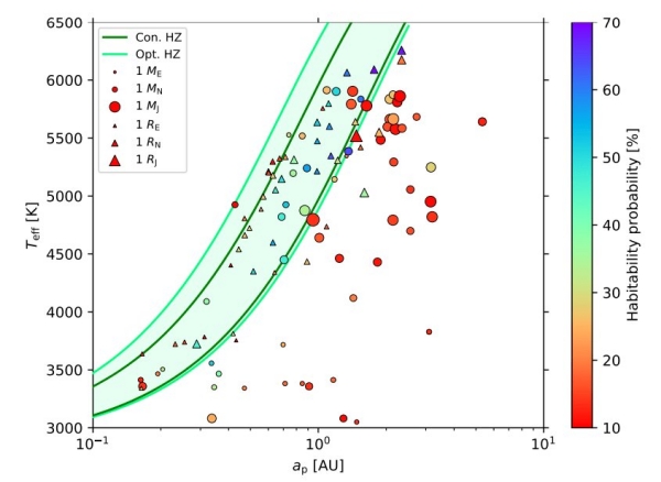
Image: This is Figure 2 from the paper. Caption: Habitability probability for exomoons around known exoplanets on the semi-major axis – stellar effective temperature plane. Planets with known masses (with or without radius data) are marked with circles, planets with known radii only are marked with triangles. Colours of the markers correspond to the fraction of habitable moons and the sizes of the markers represent the sizes of the planets as shown in the legend. Note that the legend only shows three
representative sizes (Earth, Neptune and Jupiter), while the size of the markers in the plot is scaled to the real size of the planets. Green curves represent the borders of the circumstellar habitable zone for a 1 Earth-mass planet: dark green for the consevative HZ (Con. HZ) and light green for the optimistic HZ (Opt. HZ). Credit: Dobos et al. 2022.
Given that the spectral type of over half of the stars in the Extrasolar Planets Encyclopedia is not listed, there is a good deal of play in these results, although the authors point to the mitigating effect of gas giant magnetospheres as shields against incoming stellar radiation for potentially habitable moons. Even so, stellar type is clearly an important factor, and it’s also noteworthy that while the paper mentions planet migration, its effects on exomoons are not under consideration. This is about as much as the authors have to say about migration:
It is likely that the giant planets in the circumstellar HZ were formed at larger distances from the star and then migrated inwards to their current orbit (see for example Morbidelli 2010). During the orbital migration they can lose some or all of their moons, especially if the moon orbit is close to the planet (Namouni 2010; Spalding et al. 2016). Depending on the physical and orbital parameters of the planet and the moon, as well as on the starting and final semi-major axes of the planet, some moons can survive this process, and new moons can also be captured during or after the migration of the planet.
Just how migration would affect the results of this study is thus an open question. What we do wind up with is what the authors consider a ‘target list’ for exomoon observations, although one replete with challenges. Most of these potential exomoons would orbit planets whose orbital period is in the hundreds of days, planets like Kepler-62f, with a 268 day period and a 53 percent habitability probability for an exomoon. This is an interesting case, as stable moon orbits are likely around this 1.38 Earth radius world. But what a tricky catch for both our exomoon detection techniques.
Because many of the planets in the target list are gas giants, we have to consider the probability that more than a single moon may orbit them, perhaps even several large moons where life might develop. That’s a scenario worth considering as well, independent emergence of life upon two moons orbiting the same exoplanet. But it’s one that will have to wait as we refine exomoon scenarios in future observations.
The paper is Dobos et al., “A target list for searching for habitable exomoons,” accepted at Monthly Notices of the Royal Astronomical Society 05 May 2022 (abstract / preprint). Thanks to my friend Antonio Tavani for the heads-up on this work.
Dyson Spheres: The White Dwarf Factor
I often think of Dyson structures around stars as surprisingly benign places, probably motivated by encountering Larry Niven’s wonderful Ringworld when it was first published by Ballantine in 1970. I was reading it in an old house in Iowa on a windy night and thought to start with a chapter or two, but found myself so enthralled that it wasn’t until several hours later that I re-surfaced, wishing I didn’t have so much to do the next day that I had to put the book aside and sleep.

I hope I’m not stretching the definition of a Dyson construct too far when I assign the name to Niven’s ring. It is, after all, a structure built by technological means that runs completely around its star at an orbit allowing a temperate climate for all concerned, a vast extension of real estate in addition to whatever other purposes its creators may have intended. That a technological artifact around a star should be benign is a function of its temperature, which makes things possible for biological beings.
But a Dyson sphere conceived solely as a collection device to maximize the civilization’s intake of stellar energy would not be built to biological constraints. For one thing, as retired UCLA astrophysicist Ben Zuckerman points out in a new paper, it would probably be as close to its star as possible to minimize its size. That makes for interesting temperatures, probably in the range of 300 K at the low end and reaching perhaps 1000 K, which sets up emissions up to 10 µm in wavelength, and as Zuckerman points out, this would be in addition to any emission from the star itself.
Zuckerman refers to such structures as DSRs, standing for Dyson spheres/rings, so I guess working Niven in here fits as well. Notice that when talking about these things we also make an assumption that seems reasonable. If civilizations are abundant in the galaxy, they are likely long-lived, and that means that stellar evolution has to be something they cope with as yellow dwarf stars, for example, turn into red giants and, ultimately, white dwarfs. The DSR concept can accommodate the latter and offers a civilization the chance to continue to use the energy of its shrunken star. Whether this would be the route such a civilization chooses is another matter entirely.
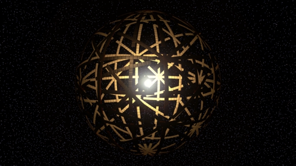
Image: Artist depiction of a Dyson swarm. Credit: Kevin McGill/Wikimedia Commons.
One useful fact about white dwarfs is that they are small, around the size of the Earth, and thus give us plenty of transit depth should some kind of artificial construct pass between the star and our telescopes. Excess infrared emission might also be a way to find such an object, although here we have to be concerned about dust particles and other potential sources of the infrared excess. Zuckerman’s new paper analyzes the observational limits we can currently derive based on these two methods.
The paper, published in Monthly Notices of the Royal Astronomical Society, uses data from Kepler, Spitzer and WISE (Wide-field Infrared Survey Explorer) as a first cut into the question, revising Zuckerman’s own 1985 work on the number of technological civilizations that could have emerged around main sequence stars that evolved to white dwarfs within the age constraints of the Milky Way. Various papers exist on excess of infrared emissions from white dwarfs; we learn that Spitzer surveyed at least 100 white dwarfs with masses in the main sequence range of 0.95 to 1.25 solar masses. These correspond to spectral types G7 and F6, and none of them turned up evidence for excess infrared emission.
As to WISE, the author finds the instrument sensitive enough to yield significant limits for the existence of DSRs around main sequence stars, but concludes that for the much fainter white dwarfs, the excess infrared is “plagued by confusion…with other sources of IR emission.” He looks toward future studies of the WISE database to untangle some of the ambiguities, while going on to delve into transit possibilities for large objects orbiting white dwarfs. Kepler’s K2 extension mission, he finds, would have been able to detect a large structure (1000 km or more) if transiting, but found none.
It’s worth pointing out that no studies of TESS data on white dwarfs are yet available, but one ongoing project has already observed about 5000, with another 5000 planned for the near future. As with K2, a deep transit would be required to detect a Dyson object, again on the order of 1000 kilometers. If any such objects are detected, we may be able to distinguish natural from artificial objects by their transit shape. Luc Arnold has done interesting work on this; see SETI: The Artificial Transit Scenario for more.
Earlier Kepler data are likewise consulted. From the paper:
From Equation 4 we see that about a billion F6 through G7 stars that were on the main sequence are now white dwarfs. Studies of Kepler and other databases by Zink & Hansen (2019) and by Bryson et al. (2021) suggest that about 30% of G-type stars are orbited by a potentially habitable planet, or about 300 million such planets that orbit the white dwarfs of interest here. If as many as one in 30 of these planets spawns life that eventually evolves to a state where it constructs a DSR with luminosity at least 0.1% that of its host white dwarf, then in a sample of 100 white dwarfs we might have expected to see a DSR. Thus, fewer than 3% of the habitable planets that orbit sun-like stars host life that evolves to technology, survives to the white dwarf stage of stellar evolution, and builds a DSR with fractional IR luminosity of at least 0.1%.
Science fiction writers will want to go through Zuckerman’s section on the motivations of civilizations to build a Dyson sphere or ring, which travels deep into speculative territory about cultures that may or may not exist. It’s an imaginative foray, though, discussing the cooling of the white dwarf over time, the need of a civilization to migrate to space-based colonies and the kind of structures they would likely build there.
There are novels in the making here, but our science fiction writer should also be asking why a culture of this sophistication – able to put massive objects built from entire belts of asteroids and other debris into coherent structures for energy and living space purposes – would not simply migrate to another star. The author only says that if the only reason to travel between the stars is to avoid the inevitable stellar evolution of the home star, then no civilization would undertake such journeys, preferring to control that evolution through technology in the home system. This gives me pause, and Centauri Dreams readers may wish to supply their own reasons for interstellar travel that go beyond escaping stellar evolution.
Also speculative and sprouting fictional possibilities is the notion that main sequence stars may not be good places to look for a DSR. Thus Zuckerman:
…main sequence stars suffer at least two disadvantages as target stars when compared to white dwarfs; one disadvantage would be less motivation to build a substantial DSR because one’s home planet remains a good abode for life. In our own solar system, if a sunshield is constructed and employed at the inner Earth-Sun Lagrange point – to counter the increasing solar luminosity – then Earth could remain quite habitable for a few Gyr more into the future. Perhaps a more important consideration would be the greater luminosity, say about a factor of 1000, of the Sun compared to a typical white dwarf.
Moreover, detecting a DSR around a main sequence star becomes more problematic. In the passage below, the term τ stands for the luminosity of a DSR measured as a fraction of the luminosity of the central star:
For a DSR with the same τ and temperature around the Sun as one around a white dwarf, a DSR at the former would have to have 1000 times the area of one at the latter. While there is sufficient material in the asteroid belt to build such an extensive DSR, would the motivation to do so exist? For transits of main sequence stars by structures with temperatures in the range 300 to 1000 K, the orbital period would be much longer than around white dwarfs, thus relatively few transits per year. For a given structure, the probability of proper alignment of orbital plane and line of sight to Earth would be small and its required cross section would be larger than that of Ceres.
So we are left with that 3 percent figure, which sets an upper limit based on our current data for the fraction of potentially habitable planets that orbit stars like the Sun, produce living organisms that produce technology, and then construct a DSR as their system undergoes stellar evolution. No more than 3 percent of such planets do so.
There is a place for ‘drilling down’ strategies like this, for they take into account the limitations of our data by way of helping us see what is not there. We do the same in exoplanet research when we start with a star, say Proxima Centauri, and progressively whittle away at the data to demonstrate that no gas giant in a tight orbit can be there, then no Neptune-class world within certain orbital constraints, and finally we do find something that is there, that most interesting place we now call Proxima b.
As far as white dwarfs and Dyson spheres or rings go, new instrumentation will help us improve the limits discussed in this paper. Zuckerman points out that there are 5000 white dwarfs within 200 parsecs of Earth brighter than magnitude 17. A space telescope like WISE with the diameter of Spitzer could improve the limits on DSR frequency derived here, its data vetted by upcoming 30-m class ground-based telescopes (Zuckerman notes that JWST is not suited, for various reasons, for DSR hunting). The European Space Agency’s PLATO spacecraft should be several times more sensitive than TESS at detecting white dwarf transits, taking us well below the 1000 km limit.
The paper is Zuckerman, “Infrared and Optical Detectability of Dyson Spheres at White Dwarf Stars,” Monthly Notices of the Royal Astronomical Society stac1113 (28 April 2022). Abstract / Preprint.

Follow with RSS or E-Mail
