Centauri Dreams
Imagining and Planning Interstellar Exploration
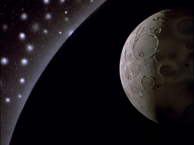
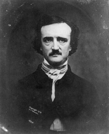
Into the Maelström
“‘This,’ said I at length, to the old man — ‘this can be nothing else than the great whirlpool of the Maelström’… The ordinary accounts of this vortex had by no means prepared me for what I saw. That of Jonas Ramus, which is perhaps the most circumstantial of any, cannot impart the faintest conception either of the magnificence, or of the horror of the scene — or of the wild bewildering sense of the novel which confounds the beholder.” So wrote Edgar Allen Poe in 1841 in a short story called “A Descent into The Maelström,” reckoned by some to be an early instance of science fiction. In today’s essay, Adam Crowl explores another kind of whirlpool, armed with the tools of mathematics to take the deepest plunge imaginable, into the maw of a supermassive black hole. Adam’s always fascinating musings can be followed on his Crowlspace site.
by Adam Crowl

The European Southern Observatory’s (ESO) GRAVITY instrument is a beam combiner in the infra-red K-band that operates as a part of the Very Large Telescope Interferometer, combining infra-red light received by four different telescopes, out of the eight operated (four 8.2 metre fixed telescopes and four 1.8 metre movable telescopes).
The latest measurements of the stars orbiting the Milky Way’s Galactic Core Super-Massive Black Hole (SMBH), otherwise known as Sagittarius A* (pronounced as ‘Sagittarius A Star’), by the GRAVITY instrument have determined its mass and distance to new levels of accuracy:
Ro = 8,275 parsecs (+\-) 9.3 parsecs and a mass of (in 106 Msol) 4.297 +\- 0.013.
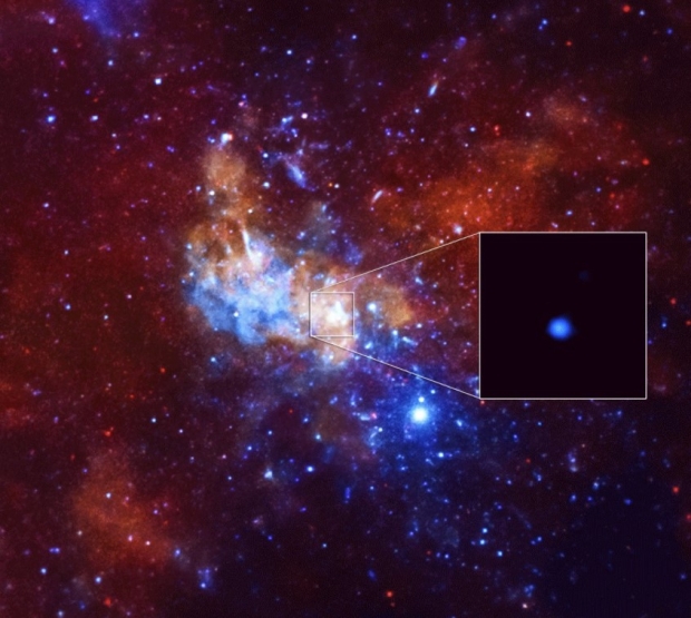
Image: The galactic centre in infrared. Credit: NASA.
In round figures, that’s 27,000 light-years and 4.3 million Solar masses. The closest that light can approach a Black Hole and still escape is the Event Horizon, which is the spherical boundary at the distance of the Schwarzschild Radius, which is a radius of 2.95325 kilometres per solar mass. Thus 4.3 million solar masses is wrapped in an Event Horizon 12.7 million kilometres in radius. In aeons to come, when the Milky Way and M31 have collided and their black holes have coalesced, the combined Super Massive Black Hole (SMBH) will mass 100 million solar masses with an event horizon almost 300 million kilometres in radius.

Image: From Tales of Mystery and Imagination, by Edgar Allan Poe, with illustrations by Arthur Rackham (1935).
Into the Maelström
Mass-energy, so General Relativity tells us, puts dents into Space-time. Most concentrations of mass-energy, like stars, planets and galaxies, form shallow dents. Black Holes – like the future SMBH – go deeper, forming an inescapable waterfall of space-time inwards to their centres, the edge of which is the Event Horizon.
Light follows the curvature of space-time, traveling the shortest pathways (geodesics). At the Event Horizon the available geodesics all point towards the “middle” of the Black Hole. For particles with rest mass, like atoms, dust and space-ships, geodesics can’t be followed, merely approached, so they follow different pathways just as inexorably towards the centre.
Instead of flying radially inwards towards the future SMBH’s Centre, let’s ponder orbiting it. For most orbital distances from any Black Hole any small mass in orbit will experience nothing different to orbiting around any other large mass. Too close and you’ll experience extreme tidal forces if the black hole is small, so to avoid being torn to shreds when approaching really close a really big Black Hole is needed. The future SMBH massing 100 million solar masses with a Schwarzschild radius of 300 million kilometres has very mild Tidal Forces at the Event Horizon, though potentially significant for things as big as stars and planets.
We have multi-year ‘movies’ of stars orbiting around our SMBH, though none as close as we will explore. Close orbits get measured in multiples of M – which is half the Schwarzschild radius. At a radius of r = 3M space-time is so curved that the geodesics form a circle around the Black Hole. Light can thus orbit indefinitely, building up to potentially extraordinary energy densities if nothing else gets in its way, forming a so-called Photon Sphere. But the centre of the Galaxy is full of dust and gas, so something is always getting in the way. Eventually even photons get so energetic they perturb each other out of the Sphere.
For particles that don’t follow geodesics, merely approximate them, the Innermost Stable Circular Orbit (ISCO) is further out, at r = 6M. Objects here travel at half the speed of light. Other shapes of orbits can dip a bit closer in, down to r = 4M. Deeper in and motion near the Black Hole is no longer “orbital”. You must point away from the Black Hole and apply thrust or in-fall is inevitable.
The equation of orbital motion from the ISCO radius (rI) all the way to the centre was only recently worked out in closed form for rotating and non-rotating (stationary) Black Holes. Previously numerical Relativity methods were used, complicating modelling of Accretion Disks around astrophysical Black Holes. The Equation of Motion of a test particle (i.e. very small mass) around a non-rotating Black Hole, which our future SMBH might approximate, is straightforward:

? is the angular distance traveled, with a range from negative infinity to zero, by convention. I’ve plotted r against ? here:
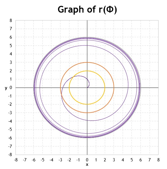
The Red Circle at r = 3 M is the Photon Sphere and the Yellow Circle at r = 2M is the Schwarzschild Radius aka Event Horizon. In this case the plot starts at r = 5.95M with the test particle circling the Black Hole 6 times before hitting the central point. The proper time experienced by an observer spiralling into the Centre is a bit more complicated. We can parameterise x as follows to make the mathematics easier:
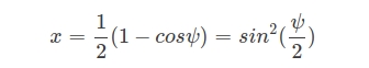
with ? running from an angle ? to 0. Then the Proper-Time ? of the inspiral trajectory is:
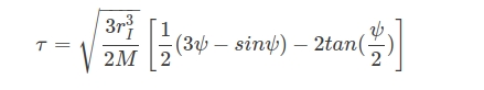
The above equation is true for any black-hole, spinning or stationary. For a stationary Black Hole, rI = 6M, so the equation simplifies to:

But what is M? It’s the “geometrised” mass of the Black Hole, which is derived by muliplying the mass by G/c2. Similarly the proper time is in units of “geometrised” time, so it needs to be divided by the speed of light, c, to convert to seconds.
In the case of the fall from r = 5.95M to r = 0, thus ? = (5.95/6) ? (?) to ? = 0, the total time is ? = 1291.14M. In the case of our Galaxy’s SMBH a proper time of M is 493 seconds. So the inspiral time is 176.6 hours and the Event Horizon is reached with 1.32 hours to go.
Surviving the Plunge
Falling into a Black Hole is probably fatal. However, like any fall, it’s not gravity that’ll kill you, but the sudden stop at the end. The final destination is the concentration of mass at the very centre. As the Centre is approached the first derivative of gravitational acceleration with respect to the radial distance vectors – the tidal forces – that will be experienced will become extreme.
Black holes are the pointy end of a spectrum of astrophysical objects. Stars exist due to their dynamic balance between the outward pressure from their fusion energy production and the inward pressure from their self gravity. When fusion energy production ends, the cores of stars begin collapsing, held above the Abyss of gravitational collapse by successive fusion energy reactions, then electron degeneracy pressure from squeezing free electrons too close together (via the Pauli Exclusion Principle), and when that isn’t enough, neutron degeneracy pressure and beyond.
Pressure is a measure of the ‘expansive’ energy packed in a volume. Dimensionally we can see that F / m2 (Pressure) = E / m3 (Energy per unit volume), so that as the mutual gravitational squeeze pushes inwards on a mass of particles which are pushing back against each other thanks to the Pauli Exclusion Principle for fermions (electrons, protons, neutrons etc) that pressure increases and increases, in a feed-back loop. Too much and equilibrium is never achieved. Thanks to Special Relativity we know that energy has mass, so that Pressure adds to the inward squeeze of gravity as particles are squeezed harder together. When the Gravity Squeeze – Push-Back Pressure process self-amplifies and runs away, the mass collapses ‘infinitely’ inwards forming a Singularity. Such a Singularity cuts itself of from the rest of the Universe when it squeezes inwards past the mass’s Schwarzschild Radius:
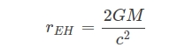
The resulting Event Horizon defines a Black Hole, by being a ‘surface of no return’ for everything, including light. Nothing escapes from within the Event Horizon. The minimum mass to cause such an inwards collapse and form a Black Hole for a mass of fermions (i.e. the same particles that make Stars, humans and space-ships) in the present day Universe is about 3 solar masses, squished into a volume smaller than 18 kilometres across.
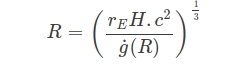
Before we get to that point there are White Dwarfs and Neutron Stars – objects supported against collapse by Electron Degeneracy Pressure and Neutron Degeneracy Pressure, respectively. White Dwarfs are typically composed of carbon and oxygen – the ashes of helium fusion – and have observed masses anywhere between 0.1 and 1.3 Solar masses. Their radius is proportional to the inverse 1/3 power of their mass:
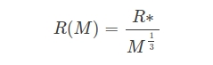
R* is a reference radius. For a cool white dwarf of 1 solar mass, the radius is about 0.8 Earth’s – 5,600 km. A space vehicle falling from infinity, on a flyby very close to such a star’s surface will rush past the lowest point of its orbit at 6,900 km/s, experiencing over 430,000 gee acceleration. In free-fall however it feels only the first derivative of that acceleration:

Which in this example is 0.15 gee per metre of radial stretching directed outwards and inwards along the direction of the radial distance to the white dwarf and a squeezing force half that directed laterally inwards from the sides. Easily resisted by small structures, like bodies and space-ships.
Neutron stars are smaller again – typically 20 km wide for a 1.3 solar mass neutron star. A near surface flyby isn’t recommended, since the tidal forces are thus almost a million times stronger. Close proximity to a magnetic neutron star is probably lethal anyway due to the intense magnetic fields long before the tidal forces rip you to shreds. Heavier neutron stars get smaller – just like white dwarfs – until they totally collapse as a black hole.
Black holes reverse the trend. The Event Horizon gets bigger linearly with their mass and there’s no upper limit to their mass. Our future Galactic SMBH’s Event Horizon will be 295.325 million kilometres in radius, give or take. Substituting the Schwarzschild Radius equation into the Tidal force equation gives us:
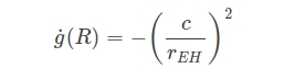
So the tidal force at the Event Horizon is 0.1 microgee per metre. The Moon could almost enter the Event Horizon peacefully…
How far into the SMBH can we, as Observers, then fall? If we can brace ourselves against 1,000 gees per metre of squeezing and stretching, then quite a long way…
Which gives a distance of 139,430 kilometres from the centre. In other words 99.953% of the way to the central Singularity.
What wonders might we see? Quantum Gravity is yet to give a clear answer. Traditionally an imploding mass ends in the Singularity, which is a geometrical point. But quantum particles can’t be reduced to a singular point and retain quantum information. A possibility, due to the massively distorted space-time around the collapsing mass, is that ultimately the quantum particles all “bounce” after hitting Planck density and explode back outwards. To external Observers this is seen, in time-dilated fashion, as the slow-leak from the Event Horizon that is Hawking Radiation. Or, if the particles “twist” in a higher dimension, so they bounce as a new Big Bang forming another Universe. This can be seen as an emergence from a White Hole, as White Holes must keep expanding else they collapse into another Black Hole.
None of those options are ‘healthy’ to be around as flesh-and-blood Observer, so presently surviving the plunge is in doubt.
As we conclude, let’s check back in with Edgar Allan Poe, who knew a few things about terrifying plunges himself. In “Descent into the Maelstrom,” he gives us a look into what might be considered a 19th Century conception of a black hole and the journey into its bizarre interior:
“Looking about me upon the wide waste of liquid ebony on which we were thus borne, I perceived that our boat was not the only object in the embrace of the whirl. Both above and below us were visible fragments of vessels, large masses of building timber and trunks of trees, with many smaller articles, such as pieces of house furniture, broken boxes, barrels and staves. I have already described the unnatural curiosity which had taken the place of my original terrors. It appeared to grow upon me as I drew nearer and nearer to my dreadful doom. I now began to watch, with a strange interest, the numerous things that floated in our company. I must have been delirious — for I even sought amusement in speculating upon the relative velocities of their several descents toward the foam below. ‘This fir tree,’ I found myself at one time saying, ‘will certainly be the next thing that takes the awful plunge and disappears,’ — and then I was disappointed to find that the wreck of a Dutch merchant ship overtook it and went down before. At length, after making several guesses of this nature, and being deceived in all — this fact — the fact of my invariable miscalculation — set me upon a train of reflection that made my limbs again tremble, and my heart beat heavily once more.”
References
Mummery, A. & Balbus, S. “Inspirals from the innermost stable circular orbit of Kerr black holes: Exact solutions and universal radial flow,” Physical Review Letters 129, 161101 (12 October 2022).
https://doi.org/10.48550/arXiv.2209.03579
Fragione, G. and Loeb, A., “An Upper Limit on the Spin of SgrA* Based on Stellar Orbits in Its Vicinity” (2020) ApJL 901 L32
DOI 10.3847/2041-8213/abb9b4

MaRMIE: The Martian Regolith Microbiome Inoculation Experiment
Alex Tolley follows up his analysis of agriculture on Mars with a closer look at the Interstellar Research Group’s MaRMIE project – the Martian Regolith Microbiome Inoculation Experiment. Growing out of discussions on methods beyond hydroponics to make the Red Planet fertile, the project is developing an experimental framework, as described below, to test our assumptions about Martian regolith here on Earth. A path forward through simulation and experiment could help us narrow the options for what may be possible for future colonists. Fertile regolith, achieved through perchlorate removal, would open up possibilities far beyond what is achievable through hydroponics.
by Alex Tolley

Successful settlement of distant locations requires living off the land, which requires resourcing food. Failure can lead to disaster, as experienced by some of the early American colonies. While near Earth space settlements could be supplied with packaged food, this would be too costly for an expanding Mars base over the long term. Food and air must be supplied from local sources, a point that has been emphasized by the Mars Society’s president, Robert Zubrin (Zubrin, 2011).
In the mid-20th century, it was assumed that agriculture on Mars would be like that on Earth, with crops growing in the Martian soil, but under clear domes to maintain air pressure, and light for photosynthesis. As a result, the focus for settlement was on the shiny technologies of transport and the design of Martian bases and cities.
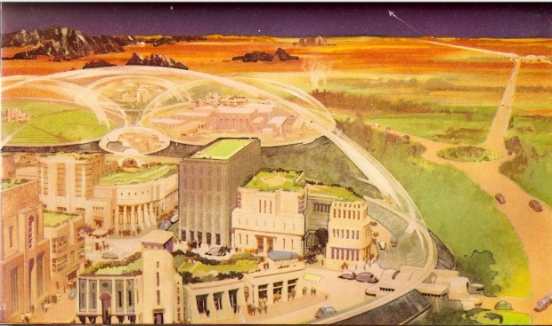
Image: The Martian Base: Painting for The Exploration of Space by Arthur C Clarke. Credit: Leslie Carr.
This rosy picture of farming on Mars was disturbed after the Apollo missions when it became apparent that plants did not grow well in lunar regolith samples. The Phoenix lander’s discovery of perchlorates on the surface of Mars meant that the Martian regolith would be toxic to plant growth without remediation. Perchlorates are found on Earth, for example in the Atacama desert, but in far lower concentrations than the 0.5-1.0% concentrations found on the surface of Mars. Perchlorates are used in industry, and the US EPA regulates perchlorate contamination because of its toxicity.
Because of the adverse nature of regolith on plant growth, the focus shifted to soilless agriculture using hydroponics or aquaponics, but as we saw in the previous post, there are limitations on the use of hydroponics. Plants with extensive root systems needed for support, especially trees, can’t be grown this way, eliminating the availability of tree fruits and nuts. Most of our grains cannot be grown using current hydroponic methods either. It really would be useful if the regolith could be altered to make it suitable for traditional agriculture, perhaps more like the farms in arid areas, such as the Middle East.
In 2022, after participating in a panel discussion on establishing a sustainable human presence on Mars at a science fiction convention (LibertyCon) in Tennessee, members of the Interstellar Research Group (IRG) including Doug Loss, Joe Meany, and Jeff Greason, considered how some experiments could be done to test how best the regolith might be treated to remove the perchlorates with bioremediation using bacteria, and convert the sterile regolith into soil suitable for agriculture. Some species of bacteria metabolize chlorates and perchlorates for energy, and therefore could be used to remediate the regolith. Relatively small, low mass cultures could be brought from Earth and exponentially cultured to meet the requirements for the volumes of regolith to be treated.
Bioremediation of perchlorate contaminated soils is established practice (Hatzinger 2005), suggesting that if it could be adapted to Martian conditions, this may be a viable solution to remove the perchlorates and solve the toxicity issue.
This use of bacteria, a low mass approach to remediate the regolith was the inspiration for core IRG members to propose a project, the Martian Regolith Microbiome Inoculation Experiment.(MaRMIE).
Mars is almost certainly too dry and cold to just irrigate the regolith on the exposed Martian surface with an inoculant of perchlorate metabolizing organisms. Knowledge about the required conditions for successful large scale regolith bioremediation, especially of temperature and pressure, was required, as well as the issue of UV and ionizing radiation.
Simulating the Martian Surface
The initial idea was to run experiments in a sealed chamber that mimicked the Martian surface environment to determine whether a terrestrial type soil might be created in which agriculture could be practiced. This Mars simulation chamber would contain a Martian regolith simulant (MRS) with added perchlorate, and inoculated with suitable bacteria. If the bacteria could break down the perchlorate, it would indicate that this approach could, in principle, be used to remediate the regolith from the surrounding area, which would then be used inside a greenhouse to grow the food crops. By doing so, the mass, complexity, and likely equipment failures of a hydroponic system could be avoided, and a more traditional agricultural approach could be practiced. This was a far more scalable solution than a technical one, allowing food production anywhere it would be needed, and was in much closer alignment with ISRU.
Early thinking was to design the experiment and have an outside PI with expertise and funding to refine the design and run the experiments. The IRG would publish a review article, and at some point participate in writing a paper on the results.
At this point, the initial group decided to invite others who might be interested in providing input and expertise to investigate the biological remediation of regolith. Of particular importance was the need to design experiments that could be done at suitable facilities. IRG hopes the guidelines that develop out of this work may be of use to anyone pursuing research into agriculture for future use on Mars, and offers them to any organization that chooses to draw on them.
Prior work had identified various bacteria that had the genes that encoded the enzymes to reduce the [per]chlorate and extract energy from it (Balk 2008, Bender 2005, Coates 2004). As the genes coding for the various enzymes for perchlorate metabolism were known it has been suggested that by just liberating the oxygen from the perchlorate the regolith could be a useful source of life support and rocket fuel oxidant (Davil 2013), therefore offering another avenue of ISRU using an engineered bacterium.
Will bioremediation need to be taken inside the base, and if so, can or should it be done as close to Martian conditions as possible, or should it be done as close to the living or working conditions, and plant growing conditions in the agricultural greenhouse? Would it be better to grow the bacteria in a bioreactor rather than in situ, or even extract the enzymes to treat the regolith, thus controlling the bacteria growth and both reducing the perchlorates and liberating the oxygen as a useful side product?
These questions can only be answered with experiments testing the various bacterial inoculants under varying conditions from terrestrial to Martian, as well as applying economic and other analyses to determine the more effective way to use bioremediation on the regolith as an initial step to making it a proactive soil for farming.
While bioremediation is one approach to removing perchlorates, the fact that they are readily water-soluble suggests that if free water is available, the regolith could be simply washed to flush out the perchlorates. This would require more plant to wash the regolith and then remove the salts to recycle the water. This method would work more effectively on regolith than soil and would not require the controlled conditions of bacterial growth and the time to build the culture.
The Phoenix lander detected the perchlorates as they deliquesced on exposure. Experiments have shown that the perchlorates will deliquesce under Martian conditions (Slank 2022).
Removal of the toxic perchlorates is just the start of the process to make the regolith fertile. There have been a number of experiments with regolith simulant to grow a variety of plants and crops under terrestrial conditions of temperature and pressure, the sort of conditions that might be expected in a Mars greenhouse that has humans managing the farm.
By far the best results have been achieved by increasing the illumination to terrestrial levels and adding carbon-rich soils to the regolith, which now will also include the many soil organisms that improve the soils. A partial solution that has also worked is to grow cover crops like alfalfa grass or reuse the waste from prior crops to be added into the regolith to improve its water retention and nutrient supply. (Kasiviswanathan 2022).
So far none of these crop growing experiments have been attempted at pressures and temperatures that differ from optimal terrestrial conditions. There is considerable space to repeat these experiments under different conditions, especially if it proves important to build structurally lighter greenhouses, or even use artificial illumination in below-ground farms, much like container farming today. While oxygen can be extracted from Martian air, water and rocks, nitrogen is less readily available, as is phosphorus. These macronutrients and the other micronutrients will have to be found and extracted to support plant growth whatever farming method is used.
As a result of all these questions, the MaRMIE project has expanded in scope beyond bioremediation, to include crop growth experiments under non-terrestrial conditions.
An Experimental Framework
The project has generated an outline of the experiments that might be done, starting with bioremediation, and extending out into the more general issue of agriculture under conditions that differ from terrestrial ones. Even this is the tip of the iceberg as gene engineered organisms might well be better adapted to conditions on Mars, reducing containment costs, nutrients, and allowing faster scale-up to support an expanding settlement.
The experimental framework encompassing the ideas to date has 4 phases:
1. Remediating perchlorates in the regolith, and any problematic chemicals produced as a result of the remediation. This requires acquiring Martian regolith simulants (MRS) and the addition of perchlorates, testing a number of bacterial and microfungal agents to remediate the MRS under terrestrial conditions, and then in stages of pressure and temperature modified towards Martian conditions.
2. Developing a microbiome tailored to Martian conditions with which to inoculate the regolith. The microbiome should lessen or remove tendencies toward cementation of the regolith as well as gradually convert it into actual soil, if possible. “Actual soil” implies the provision of required nutrients for plant growth. This includes testing microbiomes to add to the MRS along with testing pioneer plant species to condition the regolith to become more like soil.
3. Testing plant growth in microbiome-inoculated regolith under Martian lighting levels and atmospheric conditions, gradually increasing the atmospheric pressure until plant growth is acceptable.
4. Continuing plant growth testing per #3, but gradually lowering ambient temperatures toward Martian levels until plant growth diminishes unacceptably.
5. Developing agricultural structures to provide appropriate conditions, with inoculated regolith, lighting levels, atmospheric pressure, and temperature levels previously determined, and with shielding from ionizing radiation.
As for output, the initial idea to publish some sort of review paper on the known issues and prior work, indicating the direction of experimental work needed, is still in process.
As noted at the outset, the IRG cannot execute these experiments and offers this work as a contribution to the field of planetary studies. IRG hopes that this framework will be seen and used as a structure for designing experiments and building on the results of previous experiments, by any researchers interested in the ultimate goal of viable large-scale agriculture on Mars.
References
Zubrin, R. (2011). The Case for Mars: The Plan to Settle the Red Planet and Why We Must. Free Press.
Kokkinidis, I. (2016) “Agriculture on Other Worlds“ https://centauri-dreams.org/2016/03/11/agriculture-on-other-worlds/
Hatzinger P.B. (2005), “Perchlorate Biodegradation for Water Treatment Biological reactors”, 240A Environmental Science & Technology / June 1, 2005. American Chemical Society.
Balk, M. (2008) “(Per)chlorate Reduction by the Thermophilic Bacterium Moorella perchloratireducens sp. nov., Isolated from Underground Gas Storage” Applied & Environmental Microbiology, Jan. 2008, p. 403–409 Vol. 74, No. 2. doi:10.1128/AEM.01743-07
Bender, K.S, et al, (2005) “Identification, Characterization, and Classification of Genes Encoding Perchlorate Reductase” Journal of Bacteriology, Aug. 2005, p. 5090–5096 Vol. 187, No. 15. doi:10.1128/JB.187.15.5090–5096.2005
Coates J.D., Achenbach, L.A. (2004) “Microbial Perchlorate Reduction: Rocket-Fueled Metabolism”, Nature Reviews | Microbiology Volume 2 | July 2004 | 569. doi:10.1038/nrmicro926
Davila A.F. et al (2013) “Perchlorate on Mars: a chemical hazard and a resource for humans” International Journal of Astrobiology 12 (4): 321–325 (2013). doi:10.1017/S1473550413000189
Slank, R. et al. (2022) “Experimental Constraints on Deliquescence of Calcium Perchlorate Mixed with a Mars Regolith Analog” The Planetary Science Journal, 3:154 (11pp), 2022 July
https://doi.org/10.3847/PSJ/ac75c4
Kasiviswanathan P, Swanner ED, Halverson LJ, Vijayapalani P (2022) Farming on Mars: Treatment of basaltic regolith soil and briny water simulants sustains plant growth. PLoS ONE. 17(8): e0272209.
https://doi.org/10.1371/journal.pone.0272209
Food production on Mars: Dirt farming as the most scalable solution for settlement
Colonies on other worlds are a staple of science fiction and an obsession for rocket-obsessed entrepreneurs, but how do humans go about the business of living long-term once they get to a place like Mars? Alex Tolley has been pondering the question as part of a project he has been engaged in with the Interstellar Research Group. Martian regolith is, shall we say, a challenge, and the issue of perchlorates is only one of the factors that will make food production a major part of the planning and operation of any colony. The essay below can be complemented by Alex’s look at experimental techniques we can use long before colonization to consider crop growth in non-terrestrial situations. It will appear shortly on the IRG website, all part of the organization’s work on what its contributors call MaRMIE, the Martian Regolith Microbiome Inoculation Experiment.
by Alex Tolley
Introduction: Food Production Beyond Hydroponics
Conventional wisdom suggests that food production in the Martian settlements will likely be hydroponic. Centauri Dreams has an excellent post by Ioannis Kokkinidis on hydroponic food production on Mars, where he explains in some detail the issues and how they are best dealt with, and the benefits of this form of food production [1]
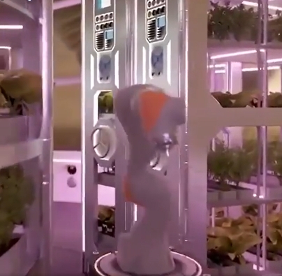
Still from a NASA video on a Mars base showing the hydroponics section.
A recent NASA short video on a very stylish possible design for a Mars base (see still above) shows a small hydroponics zone in the base, although its small size and what looks like all lettuce production would not be sufficient to feed one person, and that is before the monotonous diet would drive the crew to wish they had at least some potatoes from Mark Watney’s stash that could be cooked in a greater variety of ways.
I would tend to agree with the hydroponic approach, as well as other high-tech methods, as these food production techniques are already being used on Earth and will continue to improve, allowing a richer food source without needing to raise animals. Kokkinidis raises the issue of animal meat production for various cuisines, but in reality, the difficulties of transporting the needed large numbers of stock for breeding, as well as the increased demand for primary food production, would seem to be a major issue. [It should be noted that US farming occupies perhaps 2% of the population, yet most commentators on Mars groups seem to think that growing food on Mars will be relatively easy, with preferred animals to provide meat. How many Mars base personnel would be comfortable killing and preparing animals for consumption, even mucking out the pens?]
Hydroponics today is used for high-value crops because of the high costs. Many crops cannot be easily grown in this way. For example, it would be very difficult to grow tree fruits and nuts hydroponically, even though tree wood would be a very useful construction material. On Earth, hydroponics gains the highly desirable much-increased production per unit area coupled with a very high energy cost. It also requires inputs from established industrial processes which would have to be set up from scratch on Mars. Should there need to be lighting as well, low-energy LEDs would be hard to manufacture on Mars and would, initially at least, be imported from Earth.
Hydroponics is attractive to those with an engineering mindset. The equipment is understood, inputs and outputs can be measured and monitored, and optimized, and it all seems of a piece with the likely complexity of the transport ships and Mars base technology. It may even seem less likely to get “dirt under the fingernails” compared to traditional farming, a feature that appeals to those who prefer cleaner technologies. Unfortunately, unlike on Earth, if a critical piece of equipment fails, it will not be easily replaceable from inventory. Some parts may be 3D printable, but not complex components, or electronics. Failure of the hydroponic system due to an irreplaceable part failure would be catastrophic and lead to starvation long before a replacement would arrive from Earth. If ever there was a need for rapid cargo transport to support a Martian base, this need for rapid supply delivery would be a prime driver [4].
Soil from Regolith
Could more traditional dirt farming work on Mars, despite the apparent difficulties and lack of fine control over plant growth? The discovery that the Martian regolith has toxic levels of perchlorates and would make a very poor soil for plants seems to rule out dirt farming. If the Gobi desert is more hospitable than Mars, then trying to farm the sands of Mars might seem foolhardy, even reckless.
However, after working on a project with the Interstellar Research Group (IRG), I have to some extent changed my mind. If the Martian regolith can be made fertile, it would open up a more scalable and flexible method to grow a greater variety of plant crops than seems possible with hydroponics. Scaling up hydroponics requires far more manufacturing infrastructure than scaling up farming with an amended regolith if regolith remediation does not require a lot of equipment.
So the key questions are how to turn the regolith into viable soil to make such a traditional farming method viable, and what does this farming buy in terms of crop production, variety, and yields?
The first problem is to remove the up to 1% of perchlorates in the regolith that are toxic to plants. While perchlorates do exist naturally in some terrestrial soils, such as the Atacama desert, they are at far lower concentrations. Perchlorates are used in some industrial processes and products (e.g. rocket propellant, fireworks), and spills and their cleanup are monitored by the Environmental Protection Agency (EPA) in the USA. Chlorates were used as weedkillers and are potent oxidizers, a feature that I used in my teenage rocket experimentation, but are now banned in the EU.
There are 2 primary ways to remove perchlorates. If there is a readily available water supply, the regolith can be washed and the water-soluble perchlorates can be flushed away. The salt can be removed from the perchlorate solution with a reverse osmosis unit, a mature technology in use for desalination and water purification today. In addition, agitation of the regolith sand and dust can be used to remove the sharp edges of unweathered grains. This would make the regolith far safer to work with, and reduce equipment failure due to the abrasive dust damaging seals and metal joints. Agitation requires the low technology of rotating drums filled with a slurry of regolith and water.
A second, and more elegant approach, is to bioremediate with bacteria that can metabolize the regolith in the presence of water [5,6,7,8]. While it would seem simple to just sprinkle the exposed Martian surface with an inoculant, this cannot work, if only because the temperature on the surface is too cold. The regolith will have to be put into more clement conditions to maintain the water temperature and at least minimal atmospheric pressure and composition. At present, it is unknown what minimal conditions would be needed for this approach to work, although we can be fairly certain that terrestrial conditions inside a pressurized facility would be fine. There are a number of bacterial species that can metabolize chlorates and perchlorates to derive energy from ionized salts. A container or lined pit of graded regolith could be inoculated with suitable bacteria and the removal of the salt monitored until the regolith was essentially free of the salt. This would be the first stage of regolith remediation and soil preparation.
There is an interesting approach that could make this a dual-use system that offers safety features. The bacteria can be grown in a bioreactor, and the enzymes needed to metabolize perchlorates extracted. It has been proposed that rather than fully metabolizing the salt to chloride, enzymes could be applied that will stop at the release of free oxygen (O2). This can be used as life support or oxidant for rocket fuel, or even combustion engines on ground vehicles. The enzymes could be manufactured by gene-engineered single-cell organisms in a bioreactor, or the organisms can be applied directly to the regolith to release the O2 [10]. The design of the Spacecoach by my colleague, Brian McConnell, and me used a similar principle. As the ship used water for propellant and hull shielding, in the case of an emergency, the water could be electrolyzed to provide life-supporting O2 for a considerable time to allow for rescue [9]. Extracting oxygen from the perchlorates with enzymes is a low-energy approach to providing life support in an emergency. A small, portable, emergency kit containing a plastic bag and vial of the enzyme, could be carried with a spacesuit, or larger kits for vehicles and habitat structures.
After the perchlorate is removed from the regolith, what is left is similar to broken and pulverized lava. It may still be abrasive, and need to be abraded by agitation as in the mechanical perchlorate flushing approach.
So far so good. It looks like the perchlorate problem is solved, we just need to know if it can be carried out under conditions closer to Martian surface conditions, or whether it is best to do the processing under terrestrial or Mars base conditions. If the bacterial/enzyme amendment can be done in nothing more than lined and covered pits, or plastic bags, with a heater to maintain water at an optimum temperature, that would be a plus for scalability. If the base is located in or near a lava tube, then the pressurized tube might well provide a lot of space to process the regolith at scale.
Like lunar regolith, it has been established that perchlorate-free regolith is a poor medium for plant growth. Experiments on Mars Regolith Simulant (MRS) under terrestrial conditions of temperature, atmospheric composition, and pressure, indicate that the MRS needs to be amended to be more like a terrestrial soil. This requires nutrients, and ideally, structural organic carbon. If just removing the perchlorates, adding nutrients, and perhaps water-retaining carbon was all that was needed, this might not be too dissimilar to a hydroponic system using the regolith as a substrate. But this is really only part of the story in making fertile soil.
Nitrogen in the form of readily soluble nitrates can be manufactured on Mars chemically, using the 1% of N2 in the atmosphere. It is also possible nitrogen rich minerals on Mars may be found too. Phosphorus is the next most important macronutrient. This requires extraction from the rocks, although it is possible that phosphorus-rich sediments also may be found on Mars.
To generate the organic carbon content in the regolith, the best approach is to grow a cover crop and then use that as the organic carbon source. Fungal and bacterial decomposition, as well as worms, decompose the plants to create humus to build soil. Vermiculture to breed worms is simple given plant waste to feed on, and worm waste makes a very good fertilizer for plants. Already we see that more organisms are going to have to be brought from Earth to ensure that decomposition processes are available. In reality, healthy terrestrial soils have many thousands of different species, ranging in size from bacteria to worms, and ideally, various terrestrial soils would be brought from Earth to determine which would make the best starting cultures to turn the remediated regolith into a soil suitable for growing crops.
Ioannis Kokkinidis indicated that Martian light levels are about the same as a cloudy European day. Optimum growth for many crops needs higher intensity light, as terrestrial experiments have shown that for most plants, increasing the light intensity to Earth levels is one of the most important variables for plant growth. This could be supplied by LED illumination or using reflective surfaces to direct more sunlight into the greenhouse or below-ground agricultural area.
One issue is surface radiation from UV and ionizing radiation. This has usually resulted in suggestions to locate crops below ground, using the surface regolith as a shield. This may not be necessary as a pressurized greenhouse with exposure to the negligible pressure of Mars’ atmosphere, could support considerable mass on its roof to act as a shield. At just 5 lbs/sq.in, a column of water or ice 10 meters thick could be supported. It would be fairly transparent and therefore allow the direct use of sunlight to promote growth, supplemented by another illumination method.
Soil is not a simple system, and terrestrial soils are rich ecosystems of organisms, from bacteria, fungi, and many phyla of small animals, as well as worms. These organisms help stabilize the ecosystem and improve plant productivity. Bacteria release antibiotics and fungi provide the communication and control system to ensure the bacterial balance is maintained and provide important growth coordination compounds to the plants through their roots. The animals feed on the detritus, and the worms also create aeration to ensure that O2 reaches the animals and aerobic fungi and bacteria.
Most high-yield, agricultural production destroys soil structure and its ecosystems. The application of artificial fertilizers, herbicides to kill weeds, and pesticides to kill insect predators, will reduce the soil to a lifeless, mineral, reverting it back to its condition before it became soil. The soil becomes a mechanical support structure, requiring added nutrients to support growth.
Some farmers are trying new ideas, some based on earlier farming methods, to restore the fertility of even poor soils. This requires careful planting schedules, maintenance of cover crops, and even no-tilling techniques that emulate natural systems. Polyculture is an important technique for reducing insect pests. Combined, these techniques can remediate poor soils, eliminate fertilizers and agricultural chemicals, improve farm profitability, and even result in higher net yields than current farm practices. [11]
Without access to industrial production of agricultural chemicals and nutrients, these experimental farming practices will need to be honed until they work on Mars.
Given we have regolith-based soil what sort of crops can be grown? Almost any terrestrial crop as long as the soil conditions, drainage, pH, and illumination can be maintained.
Unlike on Earth where crops are grown where the conditions are already best, on Mars, it might well be that the crops grown will be part of a succession of crops as the soil improves. For example, in arid regions, millet is a good crop to grow with limited water and nutrients as it grows very easily under poor conditions. Ground cover plants to provide carbon and that fix nitrogen might well be a rotation crop to start and maintain the soil amendment. As the soil improves, the grains can be increased to include wheat and maize, as well as barley. With sufficient water, rice could be grown. None of these crops require pollinators, just some air circulation to ensure pollination.
For proteins, legumes and soy can be grown. These will need pollinating, and it might well be worth maintaining a greenhouse that can include bees. Keeping this greenhouse isolated will prevent bees from escaping into the base. As most of our foods require insect pollination, root crops like potatoes, carrots, and turnips, can be grown, as well as leafy greens like lettuce, and cabbage. The pièce de résistance that dirt farming allows is tree crops. A wide variety of fruit and nuts can be grown. Pomegranates are particularly suited to arid conditions. The leaf litter from such deciduous trees will be further input to improve the soil.
So the soil derived from regolith should allow a wider variety of crops to be grown, and with this, the possible variety of cuisine dishes can be supported. Food is an important component of human enjoyment, and the variety will help to keep morale high, as well as provide an outlet for prospective cooks and foodies.
Are there other benefits? As any gardener knows, growing food in the dirt is less time-consuming than hydroponics as the system is more stable, self-correcting, and resilient. This should allow for more time to be spent on other tasks than constantly maintaining a hydroponic system, where a breakdown must be fixed quickly to prevent a loss.
Meat production is beyond the scope of this essay. I doubt it will be of much importance for two main reasons. Meat production is a very inefficient use of energy. It is far better to eat plants directly, rather than convert them to meat and lose most of the captured energy. The second is the difficulty of transporting the initial stocks of animals from Earth. The easiest is to bring the eggs of cold-blooded animals (poikilotherms) and hatch them on Mars. Invertebrates and perhaps fish will be the animals to bring for food. If you can manage to feed rodents like rabbits on the ship, then rabbits would be possible. But sheep, goats, and cows are really out of the question. A million-resident city might best create factory meat from the crops if the needed ingredients can be imported or locally manufactured. My guess is that most Mars settlers will be Vegetarian or Vegan, with the few flexitarians enjoying the occasional fish or shrimp-based meal.
If you have read this far, it should be obvious that dirt farming sustainably, is not simple, nor is it easy or quick. A transport ship carrying settlers to Mars will have to supply food to eat until the first food crops can be grown. That food will likely be some variant of the freeze-dried, packaged food eaten by astronauts. Hopefully, it will taste a lot better. The fastest way to grow food crops will be hydroponics. All the kit and equipment will have to be brought from Earth. With luck, this system will reduce the demand for packaged food and become fairly sustainable, although nutrients will have to be supplied, nitrogen in particular. I don’t see sacks of nitrogen fertilizer being brought down to the surface, but instead, there may be a chemical reactor to extract the nitrogen in the Martian air and either create ammonia or nitrates for the hydroponic system.
But if the intention, as Musk aims, is to make Mars a second home, starting with 1 million residents, the size of the population that is large enough to provide the skills for modern civilization, then food production is going to need to be far more extensive than a hydroponics system in every dome or lava tube. The best way is to grow the soil as discussed above. This will not be quick and may take years before the first amended regolith becomes rich loamy, fertile soil. The sterile conditions on Mars mean that there will be no free ecosystem services. Every life form will have to originate on Earth and be transported to Mars. But life replicates, and this replication is key to success in the long term. There will be a mixture of biodiverse allotments and tracts of large-scale arable farming. Without some new technology to deflect ionizing radiation, the Martian sunlight will probably need to be indirect and directed to the crops protected by mass shields. Every square meter of Martian sunlight will only be able to support ½ a square meter of crops, so there may need to be an industry manufacturing polished metal mirrors to collect the sunlight and redirect it.
Single-cells for artificial food
Although our sensibilities suggest that the Martian settlers will want real food grown from recognizable food crops, this may be a false assumption. In the movie 2001: A Space Odyssey, Kubrick ignored Clarke’s description in his novel of how food was provided and eaten, with the almost humorous showing of liquid foods with flavors served to Heywood Floyd on his trip to the Moon.

Still from the movie 2001: A Space Odyssey. The flight attendant (Penny Brahms) is bringing the flavored, liquid food trays to the passenger and crew.
Because the Moon does not have terrestrial day-night cycles, the food was single-celled and likely grown in vats, then processed to taste like the foods they were substituting for.
Michaels: Anybody hungry?
Floyd: What have we got?
Michaels: You name it.
Floyd: What’s that, chicken?
Michaels: Something like that.
Michaels: Tastes the same anyway.
Halvorsen: Got any ham?
Michaels: Ham, ham, ham..there, that’s it.
Floyd: Looks pretty good
Michaels: They are getting better at it all the time.
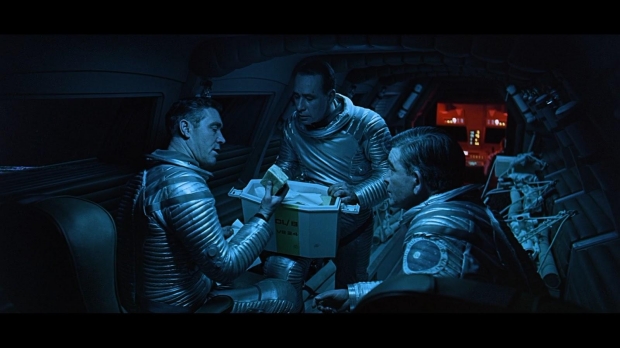
Still from the movie 2001: A Space Odyssey. Floyd and the Clavius Base personnel select sandwiches made from processed algae. Above is the conversation Floyd (William Sylvester) has with Halvorsen (Robert Beatty) and Michaels (Sean Sullivan) on the moon bus on his way to TMA1.
This is where food technology is currently taking us.
Single-cell protein has been available since at least the 18th century with edible yeast. Marmite or Vegemite is a savory, yeast-based, food spread that is an acquired taste. Today there is revived interest in various forms of SCP, some of which are commercially available for consumers, such as Quorn made from the micro-fungus, Fusarium venenatum. The advantage of single cells is that the replication rate is so high that the raw output of bacterial cells can be more than doubled daily. The technology, at least on Earth, could literally reduce huge tracts of agricultural land use, especially of meat animals. However, it does require all the inputs that hydroponic systems require, and further processing to turn the cells into palatable foods including simulated meats. Should such single-cell food production become the basic way to ensure adequate calories and food types for settlers, I suspect that real food will be as desirable as it was for Sol Roth and Detective Thorn in Soylent Green.

Still from the movie Soylent Green. Sol Roth (Edward G. Robinson) bites into an apple, stolen by Detective Thorn (Charlton Heston), that he hasn’t tasted in many years since terrestrial farming collapsed.
Physical and Mental Health with Soil
However, even if single-cell bioreactors, food manufacturing, and hydroponics do become the main methods of providing food, that does not mean that creating fertile soils from the regolith is a waste of effort. Surrounded by the ochres of the Martian landscape, the desire to see green and vegetation may be very important for mental health. Soils will be wanted to grow plants to create green spaces, perhaps as lavish as that in Singapore’s Changi Airport. Seeds brought from Earth are a low-mass cargo that can exploit local atoms to create lush landscaping for the interior of a settlement.
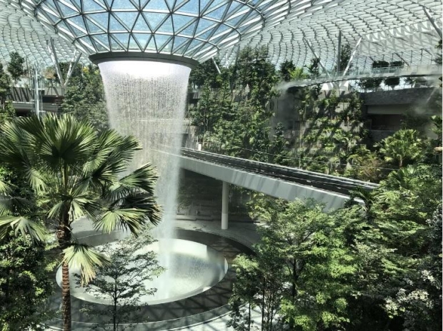
Changi Airport, Singapore. A luxurious and restful interior space of tropical plants and trees.
There is a tendency to see life on Mars not just as a blank canvas to start afresh, but also as a sterile world free of diseases and other biological problems associated with Earth. Asimov’s Elijah Bailey stories depicted “germ-free” Spacers as healthier and far longer-lived than Earthmen In their enclosed cities. We now know that our bodies contain more bacterial cells than our mammalian cells. We cannot live well without this microbiome that helps us withstand disease, digest our foods, and even influence our brain development. There is even a suggestion that children that have not been exposed to dirt become more prone to allergies later in life. Studies have shown that most animals have a microbiome with varying numbers of bacterial species. As Mars is sterile, at least as regards a rich terrestrial biosphere, it might well make sense to “terraform” it at least within the settlement cities. Creating soils that will become reservoirs for bacteria, fungi, and a host of other animal species will aid human survival and may become a useful source of biological material for the settlers’ biotechnology.
If Mars is to become a second home for humanity, it will need more people than the villages and small towns that the historical migrants to new lands create. The needed skills to make and repair things are vastly larger than they were less than two centuries ago. Technology is no longer limited to artisans like carpenters, wheelwrights, and blacksmiths, with more complex technology imported from the industrial nations. Now technologies depend on myriad specialty suppliers and capital-intensive factories. Mars will need to replicate much of this in time, which requires a large population with the needed skills. A million people might be a bare minimum, with orders more needed to be largely self-sufficient if the population is to be the backup for a possible future extinction event on Earth. Low-mass, high-value, and difficult-to-manufacture items will continue to be imported, but much else will best be manufactured locally, with a range of techniques that will include advanced additive printing. But some technologies may remain simple, like the age-old fermentation vats and stills. After all, how else will the settlers make beer and liquor for partying on Saturday nights?
References:
Kokkinidis, I (2016) “Agriculture on Other Worlds” https://centauri-dreams.org/2016/03/11/agriculture-on-other-worlds/
Kokkinidis, I (2016) “Towards Producing Food in Space: ESA’s MELiSSA and NASA’s VEGGIE”
https://centauri-dreams.org/2016/05/20/towards-producing-food-in-space-esas-melissa-and-nasas-veggie/
Kokkinidis, I (2017) “Agricultural Resources Beyond the Earth” https://centauri-dreams.org/2017/02/03/agricultural-resources-beyond-the-earth/
Higgins, A (2022) “Laser Thermal Propulsion for Rapid Transit to Mars: Part 1”
https://centauri-dreams.org/2022/02/17/laser-thermal-propulsion-for-rapid-transit-to-mars-part-1/
Balk, M. (2008) “(Per)chlorate Reduction by the Thermophilic Bacterium Moorella perchloratireducens sp. nov., Isolated from Underground Gas Storage” Applied and Environmental Microbiology, Jan. 2008, p. 403–409 Vol. 74, No. 2
https://journals.asm.org/doi/10.1128/AEM.01743-07
Coates J.D., Achenbach, L.A. (2004) “Microbial Perchlorate Reduction: Rocket-Fueled Metabolism”, Nature Reviews | Microbiology Volume 2 | July 2004 | 569
doi:10.1038/nrmicro926
Hatzinger P.B. &2005) , “Perchlorate Biodegradation
for Water Treatment Biological reactors”, 240A Environmental Science & Technology / June 1, 2005 American Chemical Society
Kasiviswanathan P, Swanner Ed, Halverson LJ, Vijayapalani P (2022) “Farming on Mars: Treatment of basaltic regolith soil and briny water simulants sustains plant growth.” PLoS ONE 17(8): e0272209.
https://doi.org/10.1371/journal.pone.0272209
Gilster, P “Spacecoach: Toward a Deep Space Infrastructure“, https://centauri-dreams.org/2016/06/28/spacecoach-toward-a-deep-space-infrastructure/
Davila A.F. et all (2013) “Perchlorate on Mars: a chemical hazard and a resource for humans” International Journal of Astrobiology 12 (4): 321–325 (2013)
doi:10.1038/nrmicro926doi:10.1017/S1473550413000189
Monbiot, G. (2022) Regenesis: Feeding the World Without Devouring the Planet Penguin ISBN: 9780143135968
An Appreciation of SETI’s Robert Gray (1948-2021)
Robert Gray was something of an outsider in the community of SETI scientists, spending most of his career in the world of big data, calculating mortgage lending patterns and examining issues in urban planning from his office in Chicago. As an independent consultant specializing in data analysis, his talents were widely deployed. But SETI was a passion more than a hobby for Gray, and he became highly regarded by scientists he worked with, many of whom were both surprised to hear of his death on December 6, 2021. It was Jim Benford who gave me the news just recently, and it humbles me to think that a Centauri Dreams post I worked with Gray to publish (How Far Can Civilization Go?) appeared just months before he died.

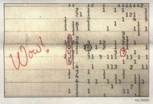
Gray’s independent status accounts for the lack of publicity about his death in our community, but I’m still startled that I’m only now learning about it. His name certainly has resonance on this site, particularly his book The Elusive Wow: Searching for Extraterrestrial Intelligence (Palmer Square Press, 2011), which should be on the bookshelf of anyone with a serious interest in SETI. The eponymous 1977 signal, received at Ohio State’s ‘Big Ear’ observatory, with Jerry Ehman’s enthusiastic ‘Wow!’ penciled in next to the printout, remains an enigma.
So obsessed was Gray with the signal – and with SETI investigation in general – that he built a radio telescope with a 12-foot dish in his backyard and pursued the work at professional installations like the Harvard/Smithsonian META radio telescope at Harvard’s Oak Ridge Observatory as well as the Very Large Array in New Mexico. He included Mount Pleasant Radio Observatory in Hobart, Tasmania in his world-spanning list of hunting grounds. His papers appeared in the likes of The Astrophysical Journal and Icarus; other essays went to such venues as Sky & Telescope, The Planetary Report, and Scientific American.
SETI has historically dealt in short ‘dwell’ times, meaning the observing instrument looks at a star and moves on so as to widen the search to as many stars as possible. Gray became interested in what would happen if we attempted long, fixed stares at high-interest stars, thus searching for signals that are intermittent as opposed to continuous. An interstellar beacon, whether targeted at specific stars or not, might send a signal that appeared and then disappeared for an arbitrary amount of time.
When I talked to Jim Benford about Gray’s work, he reminded me of his own prediction that the Wow Signal would never repeat. Interstellar applications of power beaming of the sort even now being investigated by Breakthrough Starshot would produce a small slew rate that would be consistent with a signal like the Wow as it moved across our sky. See Was the Wow Signal Due to Power Beaming Leakage for more, where Jim notes that:
The power beaming explanation for the Wow! accounts for all four of the Wow! parameters: the power density received, the duration of the signal, its frequency, and the reason why the Wow! has not occurred again. The Wow! power beam leakage hypothesis gets stronger the longer that listening for the Wow! to recur doesn’t observe it repeat.
Jim discussed power beaming as an option to explain the signal with Gray, who evidently found it one of several feasible explanations. When I first discussed it with Gray a few years back, he told me that a terrestrial explanation couldn’t be ruled out, but he found it hard to come up with a plausible one. On the phone with Jim Benford last night, I learned that Gray felt the signal was deeply enigmatic. The idea that we might never know what it was, as per Jim’s idea, would have deepened the mystery.

As to a terrestrial origin for the enigmatic reception, we would have to explain a signal that appeared at 1.42 GHz, while the band from 1.4 to 1.427 GHz is protected internationally – no emissions allowed. Aircraft can be ruled out because they would not remain static in the sky; moreover, the Ohio State observatory had excellent RFI rejection. You can see why the Wow! Signal retains its interest after all these years (see The Elusive Wow for much more). If power beaming is indeed in use in the galaxy, we may find SETI happening upon many such one-off signals as they sweep past, without serious hope of ever pinning them down to a definite source.
Power beaming aside, Gray was quite interested in intermittency as an antidote to the idea that we should look primarily for continuous isotropic broadcast signals. In a 2020 paper on the matter, he wrote:
…reducing the duty cycle to 1% could provide a 100-fold reduction in average power required, perhaps radiating for 1 s out of every 100 s. Searches observing targets for a matter of minutes might detect such signals, such as the Ohio State and META transit surveys which observed objects for 72 s and 120 s respectively, or Breakthrough Listen observing targets for three five minute periods…, or a targeted search such as Phoenix observing objects for 1,000 s in each of several spectral windows…, or the ATA observing for 30 minutes… Reducing duty cycle further yields further savings—for example a 10-4 duty cycle with a 104 reduction in average power might result in a 1 s signal every three hours, but most searches to date would be likely to miss such signals. Assuming longer signal duration does not help much; a 1-hour signal present every 100 or 10,000 hours would be very unlikely to be found by most current search strategies unless the population of such signals is large.
Gray had an excellent reputation among radio astronomers for the quality of his work; he was independent, disliked self-promotion (and particularly social media), and remained dogged in the pursuit of high-quality data. David Kipping (Columbia University), who worked with Gray on a recent paper in Monthly Notices of the Royal Astronomical Society, remembered him this way in an email this morning:
“I didn’t know Robert well, we only interacted virtually. I can say that I found his passion and persistence of the Wow signal to be an inspiration and reminded me that often the scientific investigative journey itself is the most valuable product of our endeavors. He’s an inspiration to amateur astronomers everywhere, a man who taught himself everything there was to know about that signal and more, and ended up using some of the largest radio telescopes in the world in pursuit of his dream. He was a gentleman to collaborate with and I only wish we’d had more time. It gives me a certain sense of satisfaction that his last paper with me demonstrated that for the Wow signal, hope still persists that it could repeat, not a lot of hope, but a little. And I think that’s a wonderful bookend to his publishing career.”
Beyond his work in SETI observations, Gray also looked at extending the familiar Kardashev scale, which ranks civilizations based on the energy they are able to use. In How Far Can Civilization Go?, which ran in these pages in 2021 and referenced an Astronomical Journal paper he had written on the subject, he noted that choosing what to look for in a SETI search depends on what we assume about the future course of a civilization and its power capabilities:
Whether any interstellar signals exist is unknown, and the question of how far civilization can go is critical in deciding what sort of signals to look for. If we think that civilizations can’t go hundreds or thousands of times further than our energy resources, then searches for broadcasts in all directions all of the time like many in progress might not succeed. But civilizations of roughly our level have plenty of power to signal by pointing a big antenna or telescope our way, although they might not revisit us very often, so we might need to find ways to listen to more of the sky more of the time.
I really admired the self-actualizing nature of Robert Gray’s scientific career. The man was a highly disciplined polymath whose academic background involved urban planning and policy, not physics, but without academic affiliation he made himself into a force in a highly specialized field and won the admiration of astronomers wherever he traveled. His papers are shrewd, thoughtful and provocative. I like what Jill Tarter told the Chicago Tribune shortly after his death. Calling Gray “larger than life,” Tarter added: “Bob was a constant. He really was intrigued and wanting to help, and he did — he actually followed through and was very forceful.”
Of the Gray papers I’ve mentioned above, his paper on SETI and intermittent reception is “Intermittent Signals and Planetary Days in SETI,” International Journal of Astrobiology 4 April 2020 (abstract). His paper on Kardashev is “The Extended Kardashev Scale,” Astronomical Journal 159, 228-232 (2020). Abstract. See also Kipping and Gray, “Could the ‘Wow’ signal have originated from a stochastic repeating beacon?” Monthly Notices of the Royal Astronomical Society Vol. 515, Issue 1 (September 2022), 1122-1129 (abstract).
The Value of LHS 475b
LHS 475b, a planet whose diameter is all but identical to Earth’s, makes news not so much because of what it is but because of what it tells us about studying the atmospheres of small rocky worlds. Credit for the confirmation of this planet goes to the NIRSpec (Near-Infrared Spectrograph) instrument aboard the James Webb Space Telescope, and LHS 475b marks the telescope’s first exoplanet catch. Data from the Transiting Exoplanet Survey Satellite (TESS) were sufficient to point scientists toward this system for a closer look. JWST confirmed the planet after only two transits.
Based on this detection, the Webb telescope is going to live up to expectations about its capabilities in exoplanet work. NIRSpec is a European Space Agency contribution to the JWST mission, and a major one, as the instrument’s multi-object spectroscopy mode is able to obtain spectra of up to 100 objects simultaneously, a capability that maximizes JWST observing time. No other spectrograph in space can do this, but NIRSpec deploys a so-called ‘micro-shutter’ subsystem developed for the instrument by NASA GSFC. Think of tiny windows with shutters, each measuring 100 by 200 microns.
The shutters operate as a magnetic field is applied and can be controlled individually. Murzy Jhabvala is chief engineer of Goddard’s Instrument Technology and Systems Division:
“To build a telescope that can peer farther than Hubble can, we needed brand new technology. We’ve worked on this design for over six years, opening and closing the tiny shutters tens of thousands of times in order to perfect the technology.”
LHS 475b is a rocky world that orbits a red dwarf some 40 light years out in Octans. The data from NIRSpec, taken on 31 August 2022, could not be clearer, as the image below shows.
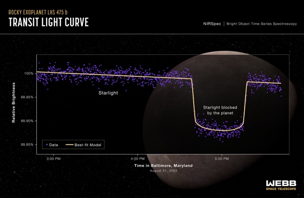
Image: This graphic shows the change in relative brightness of the star-planet system at LHS 475 spanning three hours. The spectrum shows that the brightness of the system remains steady until the planet begins to transit the star. It then decreases, representing when the planet is directly in front of the star. The brightness increases again when the planet is no longer blocking the star, at which point it levels out.] Credit: NASA, ESA, CSA, L. Hustak (STScI), K. Stevenson, J. Lustig-Yaeger, E. May (Johns Hopkins University Applied Physics Laboratory), G. Fu (Johns Hopkins University), and S. Moran (University of Arizona).
Transmission spectroscopy – applying the NIRSpec capabilities to the spectrum of starlight passing through the planet’s atmosphere during ingress and egress from a transit – should give us the opportunity to analyze the components of that atmosphere, assuming one is present. That work is ongoing but promising, as the scientists in a team led by Kevin Stevenson and Jacob Lustig-Yaeger (Johns Hopkins University Applied Physics Laboratory) pursue their investigation. JWST’s sensitivity to a range of molecules is clear, and the researchers have been able to rule out a methane-dominated atmosphere, while a compact envelope made up entirely of carbon dioxide remains a possibility. Additional spectra will be taken this summer.
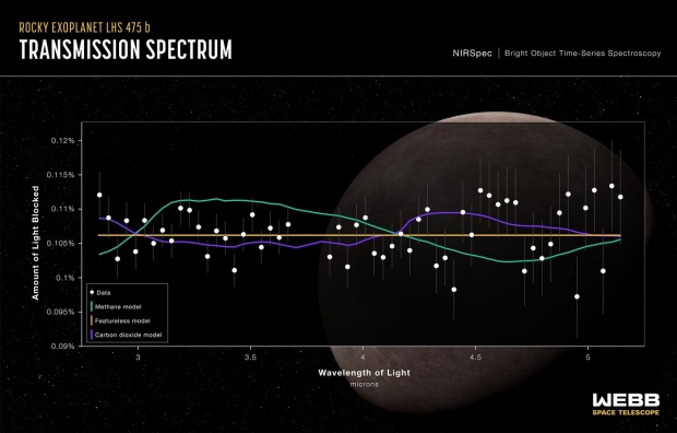
Image: The graphic shows the transmission spectrum of the rocky exoplanet LHS 475b. The data points are plotted as white circles with grey error bars on a graph of the amount of light blocked in percent on the vertical axis versus wavelength of light in microns on the horizontal axis. A straight green line represents a best-fit model. A curvy red line represents a methane model, and a slightly less curvy purple line represents a carbon dioxide model.] Credit: NASA, ESA, CSA, L. Hustak (STScI), K. Stevenson, J. Lustig-Yaeger, E. May (Johns Hopkins University Applied Physics Laboratory), G. Fu (Johns Hopkins University), and S. Moran (University of Arizona).
Given that LHS 475b orbits its star in two days, it’s no surprise to learn that the planet is considerably warmer than Earth even though it orbits an M-dwarf. We may well be looking at a Venus analogue, if an atmosphere does turn out to be present.
Bear in mind as JWST pushes into this area that M-dwarfs are prone to flares, especially in their earlier stages of development, and thus raise the question of whether a thick and detectable atmosphere can survive. LHS 475b may help us find out. The signs are promising, as the paper notes:
…our non-detection of starspot crossings during transit and the lack of stellar contamination in the transmission spectrum are promising signs in this initial reconnaissance of LHS 475b. These findings indicate that additional transit observations of LHS 475b with JWST are likely to tighten the constraints on a possible atmosphere. A third transit of LHS 475b is scheduled as part of this program (GO 1981) in 2023. An alternative path to break the degeneracy between a cloudy planet and an airless body is to obtain thermal emission measurements of LHS 475b during secondary eclipse because an airless body is expected to be several hundred Kelvin hotter than a cloudy world and will therefore produce large and detectable eclipse depths at JWST’s MIRI wavelengths… Our findings only skim the surface of what is possible with JWST.
The paper is Lustig-Yaeger et al., “A JWST transmission spectrum of a nearby Earth-sized exoplanet,” in process at Nature Astronomy (preprint).
Sunvoyager’s Pedigree: On the Growth of Interstellar Ideas
Kelvin Long’s new paper on the mission concept called Sunvoyager would deploy inertial confinement fusion, described in the last post, to drive a spacecraft to 1000 AU in less than four years. The number pulsates with possibilities: A craft like this would move at 325 AU per year, or roughly 1500 kilometers per second, ninety times the velocity of Voyager 1. This kind of capability, which Long thinks we may achieve late in this century, would open up all kinds of fast science missions to the outer planets, the Kuiper Belt, and even the inner Oort Cloud. And the conquest of inertial confinement methods would open the prospect for later, still faster missions to nearby stars.
Sunvoyager draws on the heritage of the Daedalus starship, that daring design conceived by British Interplanetary Society members in the 1970s, but as we saw last time, inertial confinement fusion (ICF) was likewise examined in a concept called Vista, and one of the pleasures of this kind of research for a scholarly sort like me is digging out the history of ideas, which in the Long paper I can trace through work in JBIS and the IEEE in the 1980s and 90s, where ICF was considered.
Vista itself appeared in the literature in the 1980s, drawing on this earlier and ongoing work, its conical shape a response to the potentially damaging neutron and x-ray flux that ICF produced. Long emulates its form factor in the Sunvoyager design. I should also mention a NASA concept called Discovery II that I hadn’t encountered until now, a spacecraft designed for a mission to the gas giants using a magnetic fusion engine. Both this and an early ICF design by Lawrence Livermore Laboratory’s Rod Hyde and colleagues in the 1970s would use an engine with a mass of 300 tons, a figure which Long selected for the calculations in his Sunvoyager paper as he validated the HeliosX code using Vista as the template: “The current level of accuracy will suffice for making predictions for the expected design performance of the Sunvoyager probe.”
So what do we get as we downselect to achieve the Sunvoyager design? The image below shows the concept.
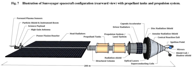
Image: This is Figure 8 in the paper. Caption: Concept design layout of Sunvoyager spacecraft configuration. Credit: Kelvin Long.
Notice the radiators, a critical part of the design, for we need to find a way to reduce waste heat. Long notes that for Vista, the radiation interaction with the structure was about 3 percent – in other words, the vehicle intercepts about that amount of the neutron and x-ray flux from the fusion reactions. He assumes a higher figure for Sunvoyager, although adding that using a mixture of deuterium and helium-3 as the fuel (Vista used a capsule of deuterium and tritium) would reduce these effects. The design also includes an annular radiation shield within the engine structure.
Long assumes the use of X-band frequencies for communications, transmitting at 8.4 GHz with a power output of 100 W, the signals to be received via the Deep Space Network’s 70-meter dishes. It’s interesting that he does not push for laser methods here, wisely so, I think, given the pointing problems we’ve discussed recently at deep space distances. Pushing data back to Earth from 1000 AU is daunting enough:
The expected data rate at 1000 AU will be 1 kBits?s. Backup medium- and low-gain antennas are also likely to be required. Note that radio signals from a distance of 1000 AU will take around 138 h to reach Earth receiving antennas, and so significant data latency should be expected. The high-gain antenna will be mounted on a rotatable fixing (rather than body mounted) and on a set of rigid extension poles so that it can always be pointed toward Earth, which avoids the need of having to rotate the entire spacecraft such as was performed for the Voyager 2 and New Horizons missions.
The Sunvoyager interstellar precursor probe would be assembled in Earth orbit following multiple launch missions. The author likens building the craft to the construction of the International Space Station, noting on the order of 10 launch vehicles may be needed to get all the parts into the assembly orbit. Booster rockets, perhaps nuclear thermal, would be used to move the vehicle away from Earth at 17 kilometers per second (which happens to be Voyager 1 speed). This reaches twice the mean Earth-Moon distance in a day or so, at which point the fusion engine can be ignited. And here we go with ICF fusion on our way to the outer Solar System:
A capsule is accelerated into the target chamber where the bank of laser beam lines can target it within the open reaction chamber to the point of thermonuclear ignition. A set of externally placed laser-focusing mirrors may be required to ensure a symmetric implosion. The plasma from the detonation will expand into the hemispherical target chamber, with the charge particles then directed by large magnetic fields internal to the chamber. These are then ejected for thrust generation while the next capsule is loaded onto the target ignition point. This occurs 10 times per second, although the hydrodynamic and nuclear phases of the ignition take place on microsecond and nanosecond time scales, respectively, so that in between each ignition there will still be around 10?5 s of time for the loading of the next capsule while the plasma from the previous one is being ejected.
The numbers on the ICF fusion for Sunvoyager are, shall we say, mind-boggling. Consider this: The mission needs 200 million fuel capsules, or 50 million per tank. This is, as the author comments, “no small undertaking,” a thought I can only echo. If we’re looking at constructing and flying a mission like this in, say, 50 years time, we may be able to assume advances in robotic automation and additive manufacturing, but we also have the problem of acquiring the needed fuel. You may recall that the Daedalus starship design was built around the notion of mining the gas giants for helium-3. That, in turn, assumes a Solar System infrastructure sufficient to make such mining feasible.
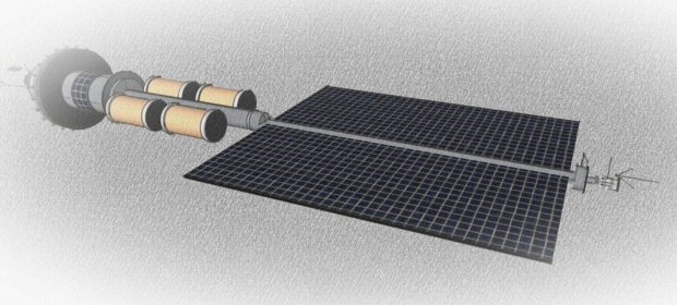
Image: This is the paper’s Figure 12. Caption: Concept design configuration (side view) of Sunvoyager spacecraft. Credit: Kelvin Long.
I like the sheer daring of concepts like Daedalus and Sunvoyager. Remember that when those frisky BIS engineers put Daedalus together, they worked at a time when it was largely considered impossible to reach another star by any means. Daedalus seemed impossible to build (it still does), but it violated no laws of physics and became a vast engineering problem. The point wasn’t that building it would bankrupt the planet. The point was that if we did decide to build it, nothing in physics would prevent it from working. Assuming, of course, that we did conquer ICF fusion for propulsion.

In other words (and Robert Forward would hammer this home again and again in talks and in papers), interstellar flight was not science fictional dreaming but a matter of reaching the appropriate level of engineering, which one day we might very well do. A mission design like Sunvoyager reminds us that we can stretch our thinking based on what we have today to make wise decisions about how and where we invest in the needed technologies. We gain scientific knowledge in doing this and we also rough out the roadmap that points to still further missions that one day reach another star.
Image: The extraordinary Robert Forward, wearing one of the trademark vests created by his wife Martha. Forward chose this photograph to appear on his own Web site.
So I think Kelvin Long is spot on in his assessment of what he does here:
Additional studies will be required to further develop the design configuration and specification for the Sunvoyager mission proposal so that it can be matured to the point of a credible mission in the coming decades to include a subsystem-level definition. However, the calculations presented in this paper show promise for what may be possible in the future provided that investments into ICF ignition physics are continued and then the applications of this technology pursued with vigor.
I think Bob Forward would have liked this paper. And because I haven’t quoted his famous lines (from JBIS in 1996) in their entirety since 2005, let me do so here. He’s looking into a future when we go from interstellar precursors into actual interstellar crossings to places like Proxima Centauri, and he sees the process:
Travel to the stars will be difficult and expensive. It will take decades of time, gigawatts of power, kilograms of energy and trillions of dollars. Recently, however, some new technologies have emerged and are under development for other purposes, that show promise of providing propulsion systems that will make interstellar travel feasible within the forseeable future — if the world community decides to direct its energies and resources in that direction. Make no mistake — interstellar travel will always be difficult and expensive, but it can no longer be considered impossible.
The paper is Long, “Sunvoyager: Interstellar Precursor Probe Mission Concept Driven by Inertial Confinement Fusion Propulsion,” Journal of Spacecraft and Rockets 2 January 2023 (full text).